Part IV. ALGEBRAIC REASONING
11. Generalizing Relationships
We have encountered many instances in this book where solving a problem numerically required numbers that we didn’t have. We often don’t know all the numbers needed to solve real problems. In some cases, the simplest way to overcome this issue is to estimate or guess a value. However, in many other cases, the value of an important quantity isn’t constant in space or time – our lack of knowledge is not a reflection of uncertainty in measurement. Instead, there is a systematic variation in the real value of a quantity and we need to allow for those changes. Under these circumstances we need to treat these quantities as variables that have unknown numerical values. Perhaps we have some idea of how large or small the numerical values can get,[1] but within these limits, the variable can take on any value.
In this new world of uncertainty, we have the tools of algebra at our disposal. At least in parts of the problem-solving process, this can be disorienting as we have to carry symbols rather than reducible values through any operations that we find necessary. However as we’ll see shortly, performing symbolic manipulations as a means to solving problems can lead to versatile and reusable solutions. What we have done prior to now can be called specializing, where we seek particular numerical values in every calculation when possible. The alternative, which you’ll recognize as a stepping-stone for algebra, is to generalize.
Writing algebraic relationships can seem to be hocus pocus at first. However, the mystique fades a bit when we remind ourselves that mathematical relationships are little more than formal logical statements. By carefully assembling what we know about quantities of interest, striving to sustain generality, and following a few tips, we can begin to use algebraic reasoning as a powerful tool for creativity and sense-making.
Writing algebraic expressions
- Identify the relevant variables and constants
- Introduce descriptive notation for each quantity
- List what is already known about each variable, using expressions with symbolic notation when possible
- Look for ways to set expressions equal to one another based on what you know; are there two ways to define the same quantity using the variables of interest?
- Guess or infer unknown relationships
- Write and simplify equated expressions as a symbolic equation
- Check for dimensional or unit consistency
When we express and manipulate equations with symbolic variables, we are doing algebra. When we state systematic relationships between symbolic variables, we’re using functions. Functions can describe derived, hypothetical, or observed relationships, depending upon how we arrive at them.
11.1 Families of Functions
In the natural and environmental sciences, a few families of functions can be used to describe relationships between key variables of interest. We will explore the most prevalent of these kinds of functions, examining their algebraic composition and the characteristics of their graphs. In the chapters that follow, we will see how functions can be used to describe relationships between measured variables and how they can be used to devise mathematical models.
Linear functions
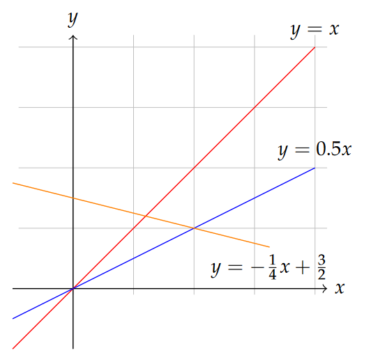
The simplest relationship between two variables—let’s call them x and y—is perhaps something like y=x. This relationship is indeed a linear relationship, stating only that y is equal to x without any modification, or that any change in the variable x results in an identical change in y. In reality, we will rarely encounter any relationships like this that are worth describing in an equation. Instead we may often find that the variables of interest are related through a constant of proportionality, call it m (might as well stick with the notation we may have seen elsewhere!).
In this case, y=mx is still a linear relationship, but now for any change in x, we expect a change in y that is m times as large as the change in x. That is what this function does for us: it converts any proposed value of x into a corresponding y according to the definition of the function. Indeed, the definition of a function in mathematics is an operation that takes a value of an explanatory or independent variable as input and produces a value for a unique response or dependent variable as output.
Here’s an example: an elephant’s tusks grow continuously with age, beginning a bit less than a year after birth. Although there is likely some variability within the population, this relationship allows biologists to estimate elephant age. Thus, a mathematical description of this relationship can be written as a linear equation:
[latex]l=ra \tag{11.1}[/latex]
where we are calling tusk length l and age a. Notice that this way of writing the relationship implies that we are treating a as an independent variable (that is, we can think of it as sort of a cause) and l is the dependent variable (an effect that depends on the cause). Depending on the circumstances, these roles could be switched. Indeed, it is easier to measure tusk length than age for a given elephant, so we might wish to use measurements of tusks to help determine the age distribution in a wild elephant population.
Also important to remember is that when we are doing science instead of just math, the variables usually have units and dimensions, which we discussed previously. If we expect our equation to be meaningful, the dimensions on the left- and right-hand sides of the equation need to be consistent (i.e. equal). So in the elephant tusk example [latex]r=l/a[/latex] is a growth rate, must have dimensions of length per time, or [ [latex]L~T^{-1}[/latex] ] (see how we get that? would that be the same if we swapped our independent and dependent variables?). If we have been measuring length in inches and age in years, our value for rr should be in inches per year.
Great! But as we said above, we might wish instead to know the age as a function of tusk length. So we need to rearrange things a bit. Let’s now define m as the number of years of age per inch of tusk length, which is just the reciprocal of r. In other words, [latex]m=1/r[/latex], which also means [latex]r=1/m[/latex]. Since we’ve just taken a reciprocal here, the dimensions of m are just the reciprocal of the dimensions of r, [ [latex]T~L^{-1}[/latex] ].
Now we can re-state our new linear relationship as [latex]l=a/m[/latex], or [latex]a=ml[/latex]. In this form, we have the dependent variable (age) on the left-hand side of the equation and the independent variable (tusk length) on the right hand side, as is convention. But at this point, what is implied about an elephant’s age if it’s tusk length is zero (l=0)? Regardless of the value of mm, plugging zero into this equation yields a=0. Of course, as mentioned above, adult tusks do not begin to develop until several months after birth. So our equation is probably not very good at representing reality (particularly for young elephants), and is therefore not yet useful. But suppose we were to change what we mean by “age” on the left-hand side. It makes sense that what we’re measuring is growth from the age when the tusks first appeared, so let’s call that age a0, which is close to 0.5 years. So the elephant age that we wish to determine is more than we would have predicted before by the an amount corresponding to the age when the tusks first appeared, a0. So our new equation, modified to account for this correction, reads:
[latex]a = a_0 + ml \tag{11.2}[/latex]
In the abstract but precise terms of mathematics, we say that a is a linear function of l with a slope of m and offset (or y-intercept) of a0. Although it seems obvious in the context of this example, the offset a0 must have dimensions of time for this equation to be meaningful.
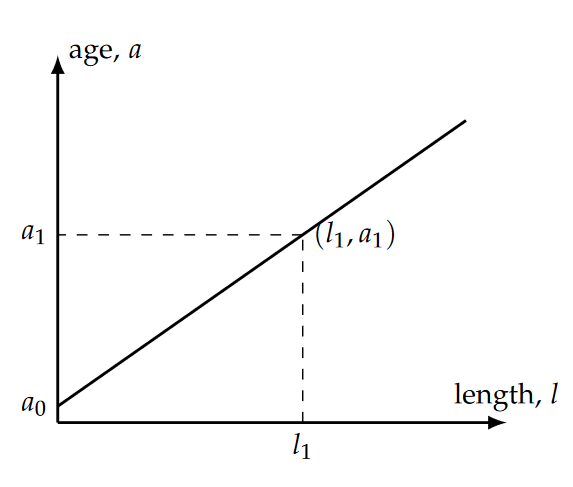
Note that the value of the growth rate, or slope m, can be determined algebraically by solving the linear equation above for m:
[latex]\large{m = \frac{a - a_0}{l},} \tag{11.3}[/latex]
which we might recognize as the “rise” of the function, [latex](a-a_0)[/latex] divided by the “run” [latex]l[/latex].
In some cases it is unnecessary, but in others we may need to specify something about the domain (a set of upper and lower constraints on the values of the independent variable) over which a proposed relationship is valid. For example, it doesn’t make sense for an elephant to have a negative age any more than it does to have a negative tusk length. There is probably an upper limit to tusk length as well, though it is hard to be confident what that might be. To be complete but conservative, we may specify that the domain of the function as 0 < [latex]l[/latex] < 160 inches. The range for our linear function is the spread of minimum to maximum values of a corresponding to the minimum and maximum values in the domain. Note that this last comment applies to linear functions (though sometimes the signs are reversed), but for some non-linear functions of interest, maximum and minimum values in the range may not correspond to maximum and minimum values bounding the domain. We’ll see examples of this later.
Functional relationships that are approximately linear are very common in the sciences. Indeed, a routine procedure in the analysis of multivariate data is linear regression, wherein the coefficients (slope and intercept) of a linear function that best fits the data are sought. Linear functions—or nonlinear ones for that matter, as we’ll see below—can also be postulated hypothetically in the construction of mathematical models.
Example: fire suppression costs (Problem 4.5)
The issue of how much suppression effort to use is at the heart of this problem, so it’s clear that suppression effort should be considered a variable. As is routine with variable quantities, we should assign a symbol to the variable and decide, at least for now, what units it will be quantified with. A single symbol is preferable (though subscripts are permissible if necessary) to prevent any ambiguity. Therefore, let’s choose the symbol E for effort, and provisionally assign the units of person-hours. A person hour has dimensions of [1 T]. Like acre-feet and other similar units, person hours is compound unit that we should understand as the number of hours worked per person multiplied by the number of people. For example, if two people work 8 hours each, that effort represents 16 person hours.
Now we need to deal with the other variable that is implied in this part of the problem: cost. First, suppose we define C as the symbol we’ll use, and US dollars as the unit of cost. Relating the cost of suppression to the effort requires some way of assigning a cost per unit of effort. Recalling our choice of units, this cost-per-unit-effort will have units of dollars per person hour, which sure sounds like an hourly wage. In fact, that’s exactly what it is! So let’s call it w. We can now state the algebraic equivalent of the sentence “suppression cost equals the number of person hours of effort times the hourly wage”. In symbols:
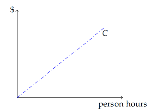
[latex]C=wE\tag{11.4}[/latex]
This equation is illustrated in Figure 11.3 as a straight line increasing from left to right. The slope of the line, analogous to mm in our abstract concept of the prototypical linear function, is w, and the y-intercept is zero. This latter observation simply articulates the (hopefully obvious) notion that the cost of zero person hours of labor should be $0.
Polynomial functions
A polynomial function is one in which the dependent variable also depends on the independent variable raised to an exponent. Polynomials are among those functions that can have multiple ups and downs in the dependent variable over the domain of the function. To refresh your memory, let’s write an abstract polynomial equation for starters:
[latex]y = b + mx + lx^2 + kx^3 + ...\tag{11.5}[/latex]
Here we have a function in which the quantities added together on the right-hand side have dependence on increasing powers of x, and the way we’ve written it we imply that the equation could go on indefinitely, incorporating ever-growing powers of x as we go. One way to describe a polynomial is by its order, which is nothing more than the integer values of the exponents of x included. If we take away the “…” from the equation above and just stop the equation after kx3, this would be a third-order polynomial, since 3 is the highest exponent of the independent variable x. Sometimes you will see the term cubic for third-order polynomials, while the term quadratic is used for second-order polynomials. To be complete, we can even pretend that the first term on the right-hand side b is really bx0, representing a “zeroth order” term.
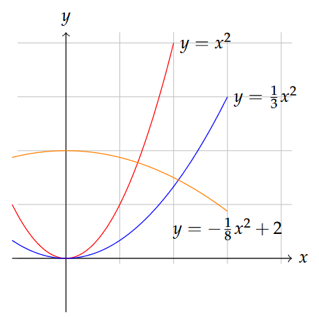
Suppose that we got rid of the l and k terms in the equation above, which we could simply do by saying that l=k=0. What’s left is just the linear function we had above, and we see now that the linear function is really a special case of a polynomial function, a “first-order polynomial”. Likewise, if b=m=k=0, we’re left with just y=lx2, a second order or quadratic polynomial. It is still a second-order polynomial if mm and b are nonzero. So you see that writing the equation as we did above allows us to imagine a polynomial of any order that we choose, and keeping or discarding any terms we wish by adjusting the lettered coefficients.
So how do these polynomial functions differ from linear functions? Take as an example the formula for the surface area of a sphere, perhaps representing a raindrop: [latex]A_s=4\pi r^2[/latex] A simple linear function as described above has a single independent variable and the values of the dependent variable depend only on the first power of the independent variable and a constant of proportionality. We can write the surface area equation as [latex]A=(4\pi r)r[/latex], and now it looks like we only have the first power of r. Great, but now our constant of proportionality contains r, so it is not a constant at all but a variable itself. So nonlinear functions are those that cannot be written as a relationship between the dependent variable and the first power of the independent variable times a constant constant of proportionality.
Before we waste too much more time talking about polynomials, I need to be clear on one thing: When we encounter polynomials in most undergraduate mathematics classes, we are only considering functions where the powers of the independent variable are whole integers. With this in mind, it is worth thinking about whether they are really useful for us. What relationships depend on integer powers of the independent variable? One area where these polynomials are useful in natural science is spatial measurement. you probably remember that the areas of squares and circles each depend on the second power of a characteristic length (side or radius). Likewise, volumes of spheres and cubes depend on the 3rd power (coincidence?). While we may never encounter perfect spheres and cubes in the natural world, we may find occasion to idealize the size and shape of something (like a sand grain, egg or raindrop as a sphere, a tree root or snake as a cylinder, etc.) in a simple model so that we can better understand something about it.
Likewise, some physical phenomena can be described with equations that depend on a whole number power (often 2) of time or position. In more complicated problems in the real world, it can also be advantageous to approximate an unruly function using a so-called series expansion of the function, which often amounts to a polynomial.
These examples notwithstanding, true polynomial functions do not arise as commonly in the natural sciences as linear and some other non-linear functions do.[2] An important exception, which we’ll grapple with quite a bit later this term, is the so-called logistic or density-dependent growth function. In ecology, this function describes the theoretical growth of populations constrained by limited space or resources. We can write the basic relationship as:
[latex]G = rN-\frac{r}{K}N^2, \tag{11.6}[/latex]
where the dependent variable G is the population growth rate [ [latex]1~T^{-1}[/latex] ], the independent variable N is the number of individuals, r is a growth constant and K is the carrying capacity. This function is quadratic because N2 is the highest power term.
Power functions
In addition to linear and polynomial functions, it is relatively common to encounter at least four other classes of functions in the natural sciences. Power functions arise commonly in ecology and geography, especially in scaling properties of organisms and habitats in space. Power functions may include any function in which the independent variable is raised to an arbitrary exponent, of the form:
[latex]y = ax^b \tag{11.7}[/latex]
The power function differs from a polynomial in that the exponent on the independent variable is not constrained to be an integer. Figure 11.5 compares the appearance of power functions with exponents greater than and smaller than 1.
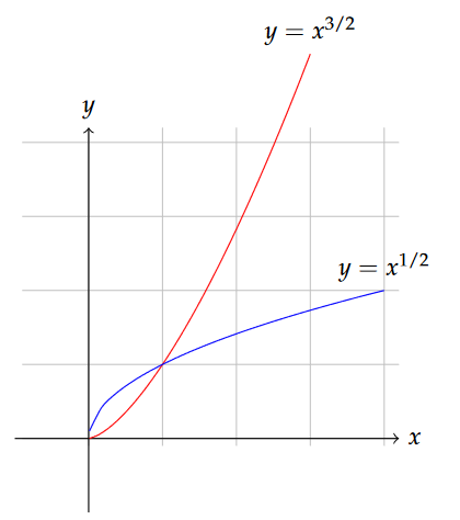
In the biological subdiscipline of island biogeography, a relationship between island area Ai and species diversity S has often been described with a power law:
[latex]S = cA_i^z \tag{11.8}[/latex]
where c is a fitting parameter and z is an exponent that is usually less than 1.
Another example of a power function appears in the description of what hydrologists call a stream’s “hydraulic geometry”, which describes how the width, depth and average velocity of a river change in time and space.[3] Channel width w, for example, typically increases downstream in a way that can be described as [latex]w=aQ^b[/latex], where Q, the water discharge, is our independent variable and a and b are empirical constants. Channel depth and velocity are described with analogous relationships.
Exponential functions
Exponential functions are different from power functions in that the independent variable appears as part of the exponent, rather than the base. A generic exponential function might look something like this:
[latex]y = a^{bx}. \tag{11.9}[/latex]
The base may often be e, which is an important (but irrational like [latex]\pi[/latex]) number close to 2.718, but needn’t be.
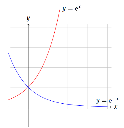
Exponential functions describe ever-increasing or ever-decreasing change, and appear in contexts like the decay of radioactive substances or unrestrained growth of populations. The radioactive decay equation might look a bit like this:
[latex]N = N_0 e^{-\lambda t} \tag{11.10}[/latex]
A similar form describes the extinction (attenuation) of sunlight with depth in a water column or forest canopy according to the Beer-Lambert law:
[latex]I = I_0 e^{-kd} \tag{11.11}[/latex]
where d is the independent variable. In addition to natural growth and decay phenomena, exponential functions appear extensively in economic analysis.
A somewhat more complicated form of exponential function is sometimes used to describe growth of individuals (fish, trees, etc.) over time. The Von Bertalanffy growth function (VBGF) can be written:
[latex]L_t = L_\infty [1-e^{-K(t-t_0)}]. \tag{11.12}[/latex]
In general, when the exponential argument is a negative number, these functions describe decay or asymptotic approach toward a limiting value. However, when the argument is positive, exponential functions describe explosive growth.
Example: fire suppression benefits (Problem 4.5)
How does a person hour of suppression effort affect the net change in timber value should fire occur? That question hasn’t been clearly answered in most settings, so there is clearly room for research on this question. But to make some headway on our problem, we may propose a relationship that makes at least some qualitative sense. If no suppression takes place, there is a risk that all the timber value is lost in the event of a fire, and that would be bad. We can also imagine that most pre-fire fuel treatments and during-fire suppression activities could reduce some of those losses, right? For example, periodic prescribed burning could reduce low fuels (forest litter, dead wood, shrubs, small trees) with only minimal of effort and little or no loss of valuable timber, resulting in perhaps a very large reduction in risk of loss to the merchantable timber. Manual thinning of the stand – again perhaps focused on the young trees and shrubs that have little timber value and introduce the greatest risk of intensifying fire—is another pre-suppression option with perhaps more effort per increment of risk reduction. At some point, however, we might imagine that additional effort has diminishing returns. While it could in theory be helpful to prune the lowest branches of dominant canopy trees to further reduce risk of intensifying fire, this would be even more costly per increment of risk reduction.
What we have described—a pattern of diminishing returns for increasing effort—could be reasonably well described with an exponential decay function, at least until we have better information. Suppose we posit then that the benefits of fire suppression effort, measured in terms of the net value change NVC, decrease as: [latex]NVC = NV_0 e^{-kE}[/latex]. Here, NV0 is the expected net value loss from a fire with no pre-fire treatments or active fire suppression efforts, and k is some constant. If NV0 has units of US dollars, the exponential term that it multiplies must have no dimensions for the equation to be homogeneous. We know from above that E has units of person hours [1 T], so k needs to have the inverse of those units to achieve homogeneity. We can interpret this constant to be a scale that defines how much returns diminish per person hour of suppression effort.
Logarithmic functions
Closely related to exponential functions are logarithmic functions. The natural logarithm, sometimes written ln\textrm{ln}, is the inverse function of e, meaning that [latex]\ln{(e^x)}=x[/latex]. The base-10 logarithm, written log10 or simply log, behaves in a similar way but for exponential functions with base 10. So [latex]\log_{10}{(10^x)}=x[/latex]. Both types of logs, and logarithms with any other base, are functions that increase rapidly for low values of the independent variable, but increase ever slower thereafter. We will find logarithms especially useful in transforming data that we suspect might be a power or exponential function, and must therefore have a basic command of the algebraic rules that apply to them. Outside of transformations and inverting exponentials, however, we won’t encounter logarithms extensively.
Exercises
- Given the description of species-area relationships given in Section on Power functions and the notion that the exponent z in Equation 11.8 is less than 1, describe what this means conceptually. How does the species diversity change with island area, and how does an increment of area change affect small islands differently than larger islands?
- Using only symbolic variables and constants, write an expression that defines that time necessary for 95% of a radioactive isotope to decay. Hint: interpret this to mean that we seek an expression for t when N/N0 = 0.05.
- Review the description of Problem 4.2. Write a hypothetical, but well-justified, algebraic equation relating the volume of herbicide needed to eliminate woody shrubs, and the basal area per unit land area of those shrubs. Consider all quantities to be variables, so use symbols rather than numbers for this.
- Review the description of Problem 4.1. Using reasonable geometric idealizations (not computer algorithms), can you write a simple algebraic equation that relates the length of a wetland’s perimeter habitat to the wetland’s area?
- For example, if we’ve used ballpark estimates and deliberately chosen high-end estimates of some of the parameters, this could provide us with an approximate upper limit on the value of the variable of interest. ↵
- But as we’ll see below, there are certainly relationships in the natural sciences where the relationships between variables are best described with functions that have non-integer exponents. ↵
- One of the scientists who developed and popularized this concept was Luna Leopold (1915-2006), the second son of Aldo Leopold. ↵

