Liquid-liquid Extraction

Monica Lamm; Laura Jarboe

3 Liquid-liquid Extraction

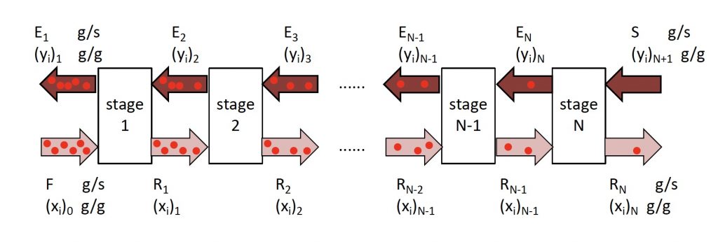
Staged Liquid-Liquid Extraction and Hunter Nash Method

$E_n$ = extract leaving stage $n$ . This could refer to the mass of the stream or the composition of the stream.

$F$ = solvent entering extractor stage 1. This could refer to the mass of the stream or the composition of the stream.

$n$ = generic stage number

$N$ = Final stage. This is where the fresh solvent S enters the system and the final raffinate $R_N$ leaves the system.

$M$ = Composition of the mixture representing the overall system. Points ( $F$ and $S$ ) and ( $E_1$ and $R_N$ ) must be connected by a straight line that passes through point $M$ . $M$ will be located within the ternary phase diagram.

$P$ = Operating point. $P$ is determined by the intersection of the straight line connecting points ( $F$ , $E_1$ ) and the straight line connecting points ( $S$ , $R_N$ ). Every pair of passing streams must be connected by a straight line that passes through point $P$ . $P$ is expected to be located outside of the ternary phase diagram.

$R_n$ = raffinate leaving stage $n$ . This could refer to the mass of the stream or the composition of the stream.

$S$ = solvent entering extractor stage $N$ . This could refer to the mass of the stream or the composition of the stream.

$S/F$ = mass ratio of solvent to feed

$(x_i)_n$ = Mass fraction of species $i$ in the raffinate leaving stage $n$

$(y_i)_n$ = Mass fraction of species $i$ in the extract leaving stage $n$

Schematic for multistage liquid-liquid extraction process. — Process schematic for multistage liquid-liquid extraction.

Determining number of stages $N$ when (1) feed rate; (2) feed composition; (3) incoming solvent rate; (4) incoming solvent composition; and (5) outgoing raffinate composition have been specified/selected.

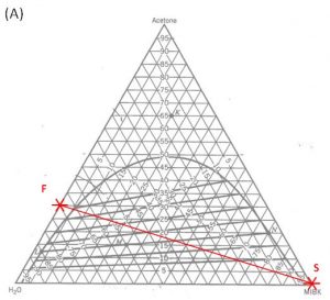
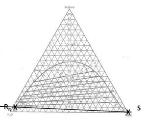
Locate points $F$ and $S$ on the ternary phase diagram. Connect with a straight line.
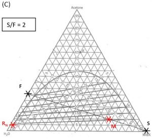
Do a material balance to find the composition of one species in the overall mixture. Use this composition to locate point $M$ along the straight line connection points $F$ and $S$ . Note the position of point $M$ .
Locate point $R_N$ on the ternary phase diagram. It will be on the equilibrium curve. Draw a straight line from $R_N$ to $M$ and extend to find the location of $E_1$ on the equilibrium curve.
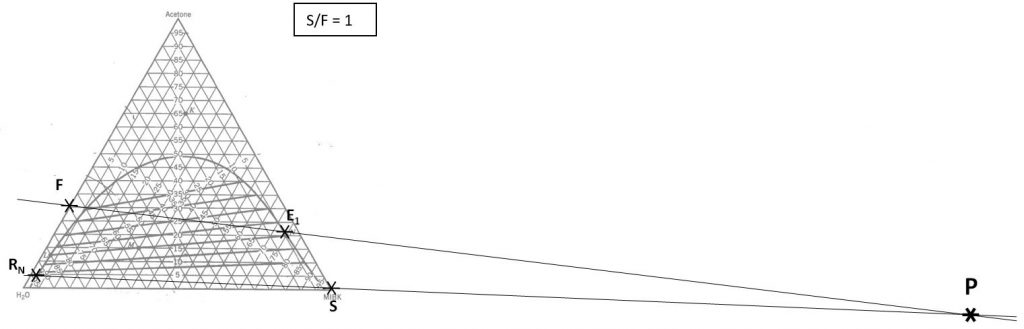
On a fresh copy of the graph, with plenty of blank space on each side of the diagram, note the location of points $F$ , $S$ , and $R_N$ (specified/selected) and $E_1$ (determined in step 3).
Draw a straight line between $F$ and $E_1$ . Extend to both sides of the diagram. Draw a second straight line between $S$ and $R_N$ . Note the intersection of these two lines and label as “ $P$ ”.
Determine the number of equilibrium stages required to achieve the desired separation with the selected solvent mass.

– Stream $R_N$ is in equilibrium with stream $E_N$ . Follow the tie-lines from point $R_N$ to $E_N$ .

– Stream $E_N$ passes stream $R_{N-1}$ . Connect point $E_N$ to operating point $P$ with a straight line, mark the location of $R_{N-1}$ .

– Stream $R_{N-1}$ is in equilibrium with stream $E_{N-1}$ . Follow the tie-lines from stream $R_{N-1}$ to $E_{N-1}$ .

– Stream $E_{N-1}$ passes stream $R_{N-2}$ . Connect $E_{N-1}$ to operating point $P$ with a straight line, mark the location of $R_{N-2}$ .

– Continue in this manner until the extract composition has reached or passed $E_{1}$ . Count the number of equilibrium stages.

Watch this two-part series of videos from LearnChemE that shows how to use the Hunter Nash method to find the number of equilibrium stages required for a liquid-liquid extraction process.

Hunter Nash Method 1: Mixing and Operating Points (9:30)
Hunter Nash Method 2: Number of Stages (6:30)

Example

1000 kg/hr of a feed containing 30 wt% acetone, 70 wt% water. The solvent is pure MIBK. We intend that the raffinate contain no more than 5.0 wt% acetone. How many stages will be required for each proposed solvent to feed ratio in the table below?

$\bold{S/F}$	$\bold{S}$ (kg/hr)	$\bold{(x_A)_M}$	target $\bold{(y_A)_1}$	$\bold{N}$
1.0
2.0
0.2

Hunter Nash Method for Finding Smin, Tank Sizing and Power Consumption for Mixer-Settler Units

Staged LLE: Hunter-Nash Method for Finding the Minimum Solvent to Feed Ratio

$E_n$ = extract leaving stage $n$ . This could refer to the mass of the stream or the composition of the stream.

$F$ = solvent entering extractor stage 1. This could refer to the mass of the stream or the composition of the stream.

$n$ = generic stage number

$N$ = Final stage. This is where the fresh solvent $S$ enters the system and the final raffinate $R_N$ leaves the system.

$M$ = Composition of the overall mixture. Points ( $F$ and $S$ ) and ( $E_1$ and $R_N$ ) are connected by a straight line passing through $M$ .

$P$ = Operating point. Every pair of passing streams must be connected by a straight line that passes through $P$ .

$R_n$ = raffinate leaving stage $n$ . This could refer to the mass of the stream or the composition of the stream.

$S$ = solvent entering extractor stage $N$ . This could refer to the mass of the stream or the composition of the stream.

$S/F$ = mass ratio of solvent to feed

$S_{\rm min}/F$ = Minimum feasible mass ratio to achieve the desired separation, assuming the use of an infinite number of stages.

$(x_i)_n$ = Mass fraction of species $i$ in the raffinate leaving stage $n$

$(y_i)_n$ = Mass fraction of species $i$ in the extract leaving stage $n$

$P_{\rm min}$ = Point associated with the minimum feasible $S/F$ for this feed, solvent and (raffinate or extract) composition. $P_{\rm min}$ is the intersection of the line connecting points ( $R_N$ , $S$ ) and the line that is an extension of the upper-most equilibrium tie-line.

Determining minimum feasible solvent mass ratio ( $S_{\rm min}/F$ ) when (1) feed composition; (2) incoming solvent composition; and (3) outgoing raffinate composition have been specified/selected.

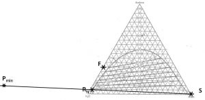
Locate points $S$ and $R_N$ on the phase diagram. Connect with a straight line.
Extend the upper-most tie-line in a line that connects with the line connecting points ( $S$ and $R_N$ ). Label the intersection $P_{\rm min}$ .
Find point $F$ on the diagram. Draw a line from $P_{\rm min}$ to F and extend to the other side of the equilibrium curve. Label $E_1$ @ $S_{\rm min}$ .
On a fresh copy of the phase diagram, label points $F$ , $S$ , $R_N$ and $E_1$ @ $S_{\rm min}$ . Draw one line connecting points $S$ and $F$ and another line connecting points $E_1$ @ $S_{\rm min}$
and $R_N$ . The intersection of these two lines is mixing point $M$ . Note the composition of species $i$ at this location.
Calculate

(5.1) $\begin{displaymath} \frac{S_{\rm min}}{F}=\frac{(x_i)_F-(x_i)_M}{(x_i)_M-(x_i)_S} \end{displaymath}$

Example

We have a 1000 kg/hr feed that contains 30 wt% acetone and 70 wt% water. We want our raffinate to contain no more than 5.0 wt% acetone. What is the minimum mass of pure MIBK required?

Liquid-Liquid Extraction: Sizing Mixer-settler Units

$\Phi_C$ = volume fraction occupied by the continuous phase

$\Phi_D$ = volume fraction occupied by the dispersed phase

$\mu_C$ = viscosity of the continuous phase (mass time^-1 length^-1)

$\mu_D$ = viscosity of the dispersed phase (mass time^-1 length^-1)

$\mu_M$ = viscosity of the mixture (mass time^-1 length^-1)

$\rho_C$ = density of the continuous phase (mass volume^-1)

$\rho_D$ = density of the dispersed phase (mass volume^-1)

$\rho_M$ = average density of the mixture (mass volume^-1)

$D_i$ = impeller diameter (length)

$D_T$ = vessel diameter (length)

$H$ = total height of mixer unit (length)

$N$ = rate of impeller rotation (time^-1)

$N_{\rm Po}$ = impeller power number, read from Fig 8-36 or Perry’s 15-54 (below) based on value of $N_{Re}$ (unitless)

$(N_{\rm Re})_C$ = Reynold’s number in the continuous phase = inertial force/viscous force (unitless)

$P$ = agitator power (energy time^-1)

$Q_C$ = volumetric flowrate, continuous phase (volume time^-1)

$Q_D$ = volumetric flowrate, dispersed phase (volume time^-1)

$V$ = vessel volume (volume)

Tank and impeller sizing

(5.2) $\begin{displaymath} {\rm residence\; time} = \frac{V}{Q_C+Q_D} \end{displaymath}$

Geometry of a cylinder

(5.3) $\begin{displaymath} V = \frac{{\pi}D_T^2H}{4} \end{displaymath}$

General guidelines

(5.4) $\begin{displaymath} \frac{H}{D_T}=1 \end{displaymath}$

(5.5) $\begin{displaymath} \frac{D_i}{D_T}=\frac{1}{3} \end{displaymath}$

Impeller power consumption:

(5.6) $\begin{equation*} P=N_{Po}N^3D_i^5{\rho}_m \end{equation*}$

(5.7) $\begin{equation*} N_{Re}=\frac{D_i^2N{\rho}_M}{{\mu}_M} \end{equation*}$

(5.8) $\begin{equation*} {\rho}_M={\rho}_C{\Phi}_C+{\rho}_D{\Phi}_D \end{equation*}$

(5.9) $\begin{equation*} {\mu}_M=\frac{{\mu}_C}{{\Phi}_C}\left[1+\frac{1.5{\mu}_D{\Phi}_D}{{\mu}_C+{\mu}_D}\right] \end{equation*}$

Modeling Mass Transfer in Mixer-Settler Units

$\Delta\rho$ = density difference (absolute value) between the continuous and dispersed phases (mass volume^-1)

$\phi_C$ = volume fraction occupied by the continuous phase

$\phi_D$ = volume fraction occupied by the dispersed phase

$\mu_C$ = viscosity of the continuous phase (mass time^-1 length^-1)

$\mu_D$ = viscosity of the dispersed phase (mass time^-1 length^-1)

$\mu_M$ = viscosity of the mixture (mass time^-1 length^-1)

$\rho_C$ = density of the continuous phase (mass volume^-1)

$\rho_D$ = density of the dispersed phase (mass volume^-1)

$\rho_M$ = average density of the mixture (mass volume^-1)

$\sigma$ = interfacial tension between the continuous and dispersed phases
(mass time^-2)

$a$ = interfacial area between the two phases per unit volume (area volume^-1)

$c_{D,\rm in}$ , $c_{D,\rm out}$ = concentration of solute in the incoming or outgoing dispersed streams (mass volume^-1)

$c^*_D$ = concentration of solute in the dispersed phase if in equilibrium with the outgoing continuous phase (mass volume^-1)

$D_C$ = diffusivity of the solute in the continuous phase (area time^-1)

$D_D$ = diffusivity of the solute in the dispersed phase (area time^-1)

$D_i$ = impeller diameter (length)

$D_T$ = vessel diameter (length)

$d_{vs}$ = Sauter mean droplet diameter; actual drop size expected to range from $0.3d_{vs}-3.0d_{vs}$ (length)

$E_{MD}$ = Murphree dispersed-phase efficiency for extraction

$g$ = gravitational constant (length time^-2)

$H$ = total height of mixer unit (length)

$k_c$ = mass transfer coefficient of the solute in the continuous phase (length time^-1)

$k_D$ = mass transfer coefficient of the solute in the dispersed phase (length time^-1)

$K_{OD}$ = overall mass transfer coefficient, given on the basis of the dispersed phase (length time^-1)

$m$ = distribution coefficient of the solute, $\Delta c_C/\Delta c_D$ (unitless)

$N$ = rate of impeller rotation (time^-1)

$(N_{\rm Eo})_C$ = Eotvos number = gravitational force/surface tension force (unitless)

$(N_{\rm Fr})_C$ = Froude number in the continuous phase = inertial force/gravitational force (unitless)

$N_{\rm min}$ = minimum impeller rotation rate required for complete dispersion of one liquid into another

$(N_{\rm Re})_C$ = Reynold’s number in the continuous phase = inertial force/viscous force (unitless)

$(N_{\rm Sh})_C$ = Sherwood number in the continuous phase = mass transfer rate/diffusion rate (unitless)

$(N_{\rm Sc})_C$ = Schmidt number in the continuous phase = momentum/mass diffusivity (unitless)

$(N_{\rm We})_C$ = Weber number = inertial force/surface tension (unitless)

$Q_D$ = volumetric flowrate of the dispersed phase (volume time^-1)

$V$ = vessel volume (volume)

Calculating $N_{\rm min}$

(6.1) $\begin{equation*} \frac{N_{\rm min}^2{\rho}_MD_i}{g{\Delta}{\rho}}=1.03\left(\frac{D_T}{D_i}\right)^{2.76}({\phi}_D)^{0.106}\left(\frac{{\mu}_M^2{\sigma}}{D_i^5{\rho}_Mg^2({\Delta}{\rho})^2}\right)^{0.084} \end{equation*}$

(6.2) $\begin{equation*} {\rho}_M={\rho}_C{\phi}_C+{\rho}_D{\phi}_D \end{equation*}$

(6.3) $\begin{equation*} {\mu}_M=\frac{{\mu}_C}{{\phi}_C}\left(1+\frac{1.5{\mu}_D{\phi}_D}{{\mu}_C+{\mu}_D}\right) \end{equation*}$

Estimating Murphree efficiency for a proposed design

Sauter mean diameter

(6.4) $\begin{equation*} {\rm if}\;\; N_{\rm We} < 10,000,\; d_{vs}=0.052D_i(N_{\rm We})^{-0.6}\exp({4{\phi}_D}) \end{equation*}$

(6.5) $\begin{equation*} {\rm if}\;\; N_{\rm We} >10,000,\; d_{vs}=0.39D_i(N_{\rm We})^{-0.6} \end{equation*}$

(6.6) $\begin{equation*} N_{\rm We}=\frac{D_i^3N^2{\rho}_C}{\sigma} \end{equation*}$

mass transfer coefficient of the solute in each phase

(6.7) $\begin{equation*} k_D=\frac{6.6D_D}{d_{vs}} \end{equation*}$

(6.8) $\begin{equation*} k_C=\frac{(N_{\rm Sh})_CD_c}{d_{vs}} \end{equation*}$

(6.9) $\begin{align*} & (N_{\rm Sh})_C = 1.237\times 10^{-5}(N_{\rm Sc})_C^{1/3}(N_{\rm Re})_C^{2/3}(\phi_D)^{-1/2}\\ & (N_{\rm Fr})_C^{5/12}\left(\frac{D_i}{d_{vs}}\right)^2 \left(\frac{d_{vs}}{D_T}\right)^{1/2}(N_{\rm Eo})_C^{5/4} \end{align*}$

(6.10) $\begin{equation*} (N_{\rm Sc})_C=\frac{{\mu}_C}{{\rho}_CD_C} \end{equation*}$

(6.11) $\begin{equation*} (N_{\rm Re})_C=\frac{D_i^2N{\rho}_C}{{\mu}_C} \end{equation*}$

(6.12) $\begin{displaymath} (N_{\rm Fr})_C=\frac{D_iN^2}{g} \end{displaymath}$

(6.13) $\begin{equation*} (N_{\rm Eo})_C=\frac{{\rho}_Dd_{vs}^2g}{{\sigma}} \end{equation*}$

Overall mass transfer coefficient for the solute

(6.14) $\begin{equation*} \frac{1}{K_{OD}}=\frac{1}{k_D}+\frac{1}{mk_C} \end{equation*}$

Murphree efficiency

(6.15) $\begin{equation*} E_{MD}=\frac{K_{OD}aV}{Q_D}\left(1+{\frac{K_{OD}aV}{Q_D}}\right)^{-1} \end{equation*}$

(6.16) $\begin{equation*} a=\frac{6\phi_D}{d_{vs}} \end{equation*}$

Experimental assessment of efficiency

(6.17) $\begin{equation*} E_{MD}=\frac{c_{D,\rm in}-c_{D,\rm out}}{c_{D,\rm in}-c^*_D} \end{equation*}$

Example

1000 kg/hr of 30 wt% acetone and 70 wt% water is to be extracted with 1000 kg/hr of pure MIBK. Assume that the extract is the continuous phase, a residence time of 5 minutes in the mixing vessel, standard sizing of the mixing vessel and impeller. Find the power consumption and Murphree efficiency if the system operates at $N_{\rm min}$ , controlled at the level of 1 rev/s. Ignore the contribution of the solute and the co-solvent to the physical properties of each phase.

MIBK
- density = 802 kg m^-3
- viscosity = 0.58 cP
- diffusivity with acetone at 25°C = 2.90×10^-9 m² s^-1
Water
- density = 1000 kg m^-3
- viscosity = 0.895 cP
- diffusivity with acetone at 25°C = 1.16×10^-9 m² s^-1
The interfacial tension of water and MIBK at 25°C = 0.0157 kg s^-2. Use the ternary phase diagram to find $m$ .

Liquid-Liquid Extraction Columns

$\Delta \rho$ = density difference (absolute value) between the continuous and dispersed phases (mass volume^-1)

$\mu_C$ = viscosity of the continuous phase (mass time^-1 length^-1)

$\rho_C$ = density of the continuous phase (mass volume^-1)

$\rho_D$ = density of the dispersed phase (mass volume^-1)

$\sigma$ = interfacial tension between the continuous and dispersed phases
(mass time^-2)

$D_T$ = column diameter (length)

$H$ = total height of column (length)

${\rm HETS}$ = height of equilibrium transfer stage (length)

$m^*_C$ = mass flowrate of the entering continuous phase (mass time^-1)

$m^*_D$ = mass flowrate of the entering dispersed phase (mass time^-1)

$N$ = required number of equilibrium stages

$u_0$ = characteristic rise velocity of a droplet of the dispersed phase (length time^-1)

$U_i$ = superficial velocity of phase $i$ (C = continuous, downward; D = dispersed, upward) (length time^-1)

$V^*_i$ = volumetric flowrate of phase $i$ (volume time^-1)

(7.1) $\begin{displaymath} U_i=\frac{4V^*_i}{{\pi}D_T^2} \end{displaymath}$

definition of superficial velocity

(7.2) $\begin{displaymath} \frac{U_D}{U_C}=\frac{m^*_D}{m^*_C}\left(\frac{{\rho}_C}{\rho_D}\right) \end{displaymath}$

(7.3) $\begin{displaymath} (U_D+U_C)_{\rm actual}=0.50(U_D+U_C)_f \end{displaymath}$

for operation at 50% of flooding

(7.4) $\begin{displaymath} u_0=\frac{0.01{\sigma}{\Delta}{\rho}}{{\mu}_C{\rho}_C} \end{displaymath}$

for rotating-disk columns, $D_T$ = 8 to 42 inches, with one aqueous phase

(7.5) $\begin{displaymath} D_T=\left(\frac{4m^*_D}{{\rho}_DU_D{\pi}}\right)^{0.5}=\left(\frac{4m^*_C}{{\rho}_CU_C{\pi}}\right)^{0.5} \end{displaymath}$

(7.6) $\begin{displaymath} H = {\rm HETS}*N \end{displaymath}$

Example

1000 kg/hr of 30 wt% acetone and 70 wt% water is to be extracted with 1000 kg/hr of pure MIBK in a 2-stage column process. Assume that the extract is the dispersed phase. Ignoring the contribution of the solute and the co-solvent to the physical properties of each phase, find the required column diameter and height.

MIBK
- density = 802 kg m^-3
- viscosity = 0.58 cP
Water
- density = 1000 kg m^-3
- viscosity = 0.895 cP
The interfacial tension of water and MIBK at 25°C = 0.0157 kg s^-2.

License

Icon for the Creative Commons Attribution-NonCommercial 4.0 International License

Chemical Engineering Separations: A Handbook for Students Copyright © 2021 by Monica H. Lamm and Laura R. Jarboe is licensed under a Creative Commons Attribution-NonCommercial 4.0 International License, except where otherwise noted.