
Chapter 4: Refresher on Population and Quantitative Genetics
Asheesh Singh; Anthony A. Mahama; and Walter Suza
The presence of genetic variation is a key prerequisite for genetic improvement in plant breeding. Creation of breeding populations with sufficient variability among individuals is key to success of breeding programs. Behind the visual variability in populations are underlying genetic variations and interactions, the understanding of which the plant breeders and students in plant breeding can benefit from to ensure successful use of the sources of genetic variation and their manipulation to maximize improvement of programs.
- Demonstrate understanding of the different populations in plant breeding
- Distinguish between qualitative and quantitative traits important in plant breeding
- Demonstrate understanding of the concept of variability, phenotype, genotype, and genotype x environment interactions
- Describe the concept of heritability and its importance in plant breeding
- Discuss selection theory and response to selection (breeder’s equation)
- Distinguish between specific versus general combining ability and their calculations
- Describe the concept of heterosis and write the equation for estimating heterosis
Populations
Basic Principles
Population genetics deals with the prediction and description of the genetic structure of populations as it relates to Mendel’s laws and other genetic principles. Fundamentals of population genetics were developed for natural outcrossing species, but it is important to note that plant breeders utilize population genetic theories because the breeding methods they use are designed to increase the frequency (proportion) of desirable alleles in the population.
The difference between population and Mendelian genetics is that population genetics principles are applied to the total products of all matings that will occur in the population, not just to one specific mating (as is the case with Mendelian genetics).
Population refers to any group of individuals sharing a common gene pool.
Gene pool refers to the sum total of all genes present in a population.
Types of Populations in Breeding Program
Simple populations
Simple populations consist of two to four parents. The simplest type of population is created by developing a segregating population from a cross of two elite lines, i.e. a two-way cross population. An F2 generation can be produced by self-fertilizing the F1. F2 and higher filial generations are developed (and selections made in these populations) in commercial breeding programs of self-fertilizing crops (such as wheat, rice, and soybean). In many cross-pollinated crops like maize, the commercially marketed products are single cross hybrids (F1) from inbred parents developed following generations of selection and selfing.
Another type of segregating population is a backcross population, which can be made from the F1 by crossing it to one of the parents, producing a BC1F1, which can be selfed to form a segregating population. The backcross population is particularly useful if one parent is superior to the other in most traits and the objective is to combine one or two genes from unadapted (or overall undesirable) parent into an elite line. Each backcross F1 seed will be heterogeneous and therefore phenotypic testing or marker-assisted selection will be required to select the desirable plant to use in subsequent backcrossing to fix or enrich for favorable genes.
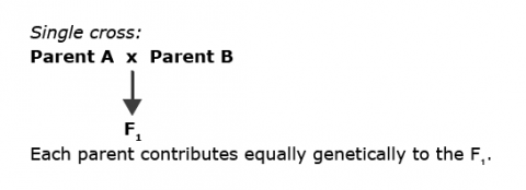
Single Cross
A cross involves two parents (Fig. 1), for example the crossing of two elite lines for F1‘s from which an F2 population can be produced by self-fertilizing the F1. Parent ‘A’ and ‘B’ contribute 50% each (genetically)
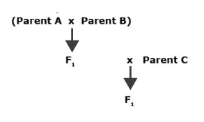
Three-Way Cross
Crossing the single cross F1 to a third parent (inbred line) and self-pollinating the resulting three-way hybrid creates a three way cross population (Fig. 2). The generation resulting from the self-fertilization is generally called the F2 population. Note that the third parent contributes 50% of the alleles to the final population therefore should generally always be one of the best parents. A three way cross is useful if one of the parents is less desirable and one or two are more desirable.
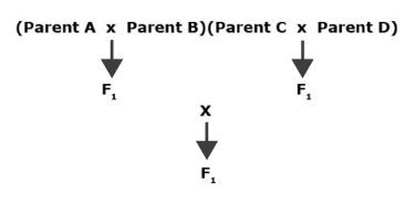
Double Cross
A double cross or four-parent cross population can be produced by crossing two single cross F1 hybrids, each formed from two inbred lines (Fig. 3). Each of the resulting individuals in the double cross generation will be genetically distinct.
Complex Populations
Some of the reasons to use complex populations include: developing good information for parents and full-sib families, identification of heterotic groups, estimation of general and/or specific combining ability, develop estimates of additive, dominant, and epistatic genetic effects and genetic correlations. Complex populations deriving from more than four parents can be constructed in several ways:
- Nested designs
- Factorial designs
- Diallel cross
- Half-diallel
- Partial diallel
- Polycrosses
Nested Designs
A North Carolina Design I (nested design) involves mating of each of the male parents to a different subset of female parents as shown in Table 1.
| n/a | Male Parent (♂) | ||||||||
|---|---|---|---|---|---|---|---|---|---|
| A | B | C | D | ||||||
| Female Parent (♀) |
1 | X | n/a | n/a | n/a | ||||
| 2 | X | n/a | n/a | n/a | |||||
| 3 | n/a | X | n/a | n/a | |||||
| 4 | n/a | X | n/a | n/a | |||||
| 5 | n/a | n/a | X | n/a | |||||
| 6 | n/a | n/a | X | n/a | |||||
| 7 | n/a | n/a | n/a | X | |||||
| 8 | n/a | n/a | n/a | X | |||||
| Note: X means “cross”. n/a means cell is blank. | |||||||||
A North Carolina Design II (factorial design), Table 2, involves mating each member of a group of males (A, B, C, D) to each member of the group of females (1, 2, 3, 4, 5, 6, 7, 8).
| n/a | Male Parent (♂) | ||||
|---|---|---|---|---|---|
| A | B | C | D | ||
| Female Parent (♀) |
1 | X | X | X | X |
| 2 | X | X | X | X | |
| 3 | X | X | X | X | |
| 4 | X | X | X | X | |
| 5 | X | X | X | X | |
| 6 | X | X | X | X | |
| 7 | X | X | X | X | |
| 8 | X | X | X | X | |
| Note: X means “cross” | |||||
| n/a | Male Parent (♂) | ||||||||
|---|---|---|---|---|---|---|---|---|---|
| A | B | C | D | ||||||
| Female Parent (♀) | 1 | X | X | X | X | ||||
| 2 | X | X | X | X | |||||
| 3 | X | X | X | X | |||||
| 4 | X | X | X | X | |||||
| 5 | X | X | X | X | |||||
| 6 | X | X | X | X | |||||
| 7 | X | X | X | X | |||||
| 8 | X | X | X | X | |||||
| Note: X means “cross”. n/a means cell is blank. | |||||||||
Diallel Cross
A diallel refers to a crossing scheme in which all pairwise crosses among the parents are made as a series of single crosses (Table 3). Diallels can be “complete,” in which crosses are made in both directions i.e., including reciprocal crosses, as well as self-pollinations of parents. In other words, each parent is mated with every parent in the population (including selfs and reciprocals).
| n/a | Male Parent (♂) | ||||||||
|---|---|---|---|---|---|---|---|---|---|
| 1 | 2 | 3 | 4 | 5 | 6 | 7 | 8 | ||
| Female Parent (♀) | 1 | X | X | X | X | X | X | X | X |
| 2 | X | X | X | X | X | X | X | X | |
| 3 | X | X | X | X | X | X | X | X | |
| 4 | X | X | X | X | X | X | X | X | |
| 5 | X | X | X | X | X | X | X | X | |
| 6 | X | X | X | X | X | X | X | X | |
| 7 | X | X | X | X | X | X | X | X | |
| 8 | X | X | X | X | X | X | X | X | |
| Note: X means “cross”. n/a means cell is blank. | |||||||||
From a breeding standpoint, selfs do not contribute any interesting recombination if the parents are inbred, and because crosses in different directions are functionally the same in terms of recombination in later generations (unless there are maternal and paternal effects), the complete diallel is usually used only as a research tool. In the example given above, Parent 1 will be selfed, as well as used as male and as female in crosses with the other parents, e.g. parent 2, thus doubling the number of crosses with parent 2, i.e. 1 x 2 and 2 x 1.
Half-Diallel Cross
In a half-diallel cross, each parent is mated with every other parent in the population excluding selfs and reciprocals (Table 4).
| n/a | Male Parent (♂) | ||||||||
|---|---|---|---|---|---|---|---|---|---|
| 1 | 2 | 3 | 4 | 5 | 6 | 7 | 8 | ||
| Female Parent (♀) | 1 | n/a | n/a | n/a | n/a | n/a | n/a | n/a | n/a |
| 2 | X | n/a | n/a | n/a | n/a | n/a | n/a | n/a | |
| 3 | X | X | n/a | n/a | n/a | n/a | n/a | n/a | |
| 4 | X | X | X | n/a | n/a | n/a | n/a | n/a | |
| 5 | X | X | X | X | n/a | n/a | n/a | n/a | |
| 6 | X | X | X | X | X | n/a | n/a | n/a | |
| 7 | X | X | X | X | X | X | n/a | n/a | |
| 8 | X | X | X | X | X | X | X | n/a | |
| Note: X means “cross”. n/a means cell is blank. | |||||||||
Partial Diallel Cross
Partial diallel refers to a crossing scheme in which only selected subsets of full diallel crosses are made (Table 5). A partial diallel could be made among a large number of parents, followed by a diallel among the single crosses, allowing for sampling more recombination events among favorable parents. This would allow incorporation of a diversity of germplasm without having to make a massive number of crosses.
| n/a | Male Parent (♂) | ||||||||
|---|---|---|---|---|---|---|---|---|---|
| 1 | 2 | 3 | 4 | 5 | 6 | 7 | 8 | ||
| Female Parent (♀) | 1 | n/a | X | X | X | n/a | n/a | n/a | n/a |
| 2 | n/a | n/a | X | X | X | n/a | n/a | n/a | |
| 3 | n/a | n/a | n/a | X | X | X | n/a | n/a | |
| 4 | n/a | n/a | n/a | n/a | X | X | X | n/a | |
| 5 | X | n/a | n/a | n/a | n/a | X | X | X | |
| 6 | X | X | n/a | n/a | n/a | n/a | X | X | |
| 7 | X | X | X | n/a | n/a | n/a | n/a | X | |
| 8 | X | X | X | X | n/a | n/a | n/a | n/a | |
| Note: X means “cross”. n/a means cell is blank. | |||||||||
Practically making crosses for a diallel (or other methods of population formation) in the field requires careful planting arrangements. There are several things to consider: such as flowering time, length of time pollen and stigma will be viable, and susceptibility to drought or pest. From a planting perspective in the field, the considerations are: (1) physical distance between parents, i.e., distance between rows or plants (how close do you want to have each of the two parents you are crossing), such as side-by-side or not; and (2) how much land area is available for the population development. Planting arrangements vary from unpaired parents, in which parents are not very close to each other but less land is required for example circular crossing (aka, chain crossing), in which parents are crossed in pairs sequentially, A x B, B x C, etc., with the final parent crossed back to A.; or paired parents, in which all parents to be crossed are grown in adjacent rows, however, a large area is required for crossing nursery.
Polycrosses
Polycrosses are used to intercross a number of selected plants. Polycrosses are primarily used for cross-pollinating crop species allowing natural conditions (e.g., wind or insects) to make the crosses. Thus, the pollen for a polycross comes from the population of selected (or unselected ) individuals as pollen parent source, and no control on the success of any particular parental pairing is known. Some plants will undoubtedly produce more pollen than others, thereby resulting in a higher percentage of pollinations than others. In a clonal crop, parent genotypes may be replicated in a manner to ensure each genotype is adjacent or surrounded by all other genotypes to provide equal frequencies of crossing among all genotypes. If sufficient land is available and not too many entries are included in the crossing, a Latin Square arrangement (each parent is present in each row and each column of the design) is a good way to enhance the equal chance of pollination among the genotypes. Another option will be a randomized complete block design if the number of parents is large. A higher number of replications are planted (two or more); however, each parental genotype will not be surrounded by all other genotypes in equal frequency therefore non-random and unequal mating occurs. A number of other aspects need to be considered for successful intercrossing which include flowering time, wind effects, and insect pollinator activity. Flowering time needs to be similar among the parents to prevent certain parents intercross more frequently (due to overlapping flowering time) than they should by random chance. For polycrosses done in the greenhouse by hand (e.g., in alfalfa), flowering can be controlled more easily than in a field planting and this is something breeders can consider using, resource permitting. If a breeder is relying on wind pollination, the dominant direction of the prevailing wind will affect pollination and lead to a non-random pollination. For insect-pollinated crops, placing bee hives near the field is often done to ensure successful pollination.
Polycross Nursery Harvest Procedures
To ensure harvested seed of the polycross is representative of seed from random and equal pollinations (which is what is intended) three major procedures exist for harvest:
- Bulk harvest the entire plot. This is the easiest method but will result in unequal contributions by both paternal and maternal parents to the population because maternal or paternal parent that produces more seed will represent a higher proportion of seed in the lot.
- If replications were used in the crossing design, bulk each parental genotype’s seed across all the replications. Composite equal amounts of seed from each parent to make the population. This is the most commonly used method but there is an element of unequal contribution. Different clones (or inbred or doubled haploid) of the same parental genotype may not produce the same amount of seed, so this method will skew the population toward the pollen parents surrounding the highest yielding maternal clone.
- One method that will overcome the problem listed in #2 above is to composite an equal amount of seed from each clone in the polycross – that is, equal amounts from each parental genotype in each replication. This method provides the most balanced contribution to the population possible. If there is a replication that didn’t perform to provide the minimum seed, some adjustments (in either among sample per replication or pulling more from other reps for that genotype) will be needed, leading to some un-equal contribution.
Qualitative and Quantitative Traits
Qualitative traits are traits that are generally controlled by a single or few genes, the expression of which have phenotype that can be classified into distinct categories. These traits are generally not influenced by environment and are recorded/scored as presence versus absence, or yes versus no, different color, seed shape type, etc. Examples include the presence of awns in wheat (awned versus awnless), flower color (purple versus white), round versus wrinkled seed (Mendel’s garden pea experiment). These traits will be in the ‘yes versus no’ classification and their expression will be the same irrespective of the environment the plants are grown, that is, genotypes with round seed will produce round seed in all environments.
Quantitative traits are controlled by several genes, whose expression produce a phenotype that cannot be classified into distinct categories, i.e., there will be a continuum of phenotypes. These traits are influenced by the environment, such that the same genotype will produce different phenotypes in different environments. Examples of such traits are yield, protein %, oil %, and seed weight.
Traits such as plant height are described as qualitative because they can be classified as short versus tall. However, it is important to note that plant height can occur across a range of values (cm) meaning that these are not innate categories and most appropriate measurement is on a numerical scale, which makes plant height a quantitative trait from a trait measurement perspective. In most crops, several plant height genes have been identified, again validating that plant height is not a truly qualitative trait.
Disease resistance can be qualitative or quantitative, and this distinction between them will be driven by genetic control, influence of environment, and phenotypic expression. Most traits that a plant breeder works to improve are quantitative.
Types of Gene Action
Expression of genes can be described as additive or non-additive (dominance or epistatic).
Additive gene action
A gene acts in an additive manner when the substitution of one allele for another allele at a particular gene locus always causes the same effect. For example,
A1A1 – A1A2 = A1A2 – A2A2
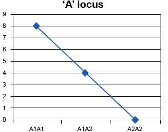
That is, for this case, the effect of substituting A1 for A2 is the same whether the substitution occurs in genotype A2A2 or in genotype A1A2 (Fig. 4, Table 1).
| A1A1 | 8 |
|---|---|
| A1A2 | 4 |
| A2A2 | 0 |
Thus the effect of substituting an A1 allele with an A2 allele is +4.
Genotypic Values at ‘B’ Locus
As shown in Table 7, if we assume genotypic values at ‘B’ locus as:
| B1B1 | 4 |
|---|---|
| B1B2 | 2 |
| B2B2 | 0 |
then, as shown in Table 8, the effect of substituting allele B1 for B2 is +1, indicating an additive effect.
| Genotype | Genotypic value |
|---|---|
| A1A1B1B1 | 12 |
| A1A1B1B2 | 10 |
| A1A1B2B2 | 8 |
| A1A2B1B1 | 8 |
| A1A2B1B2 | 6 |
| A1A2B2B2 | 4 |
| A2A2B1B1 | 4 |
| A2A2B1B2 | 3 |
| A2A2B2B2 | 0 |
When a gene acts additively, the maximum trait expression will occur in the genotype which possesses all the “favorable” alleles.
Non-additive Gene Action
Non-additive gene action results from the effects of dominance (intra-locus interactions, i.e. A1/A2) and/or the effects of epistasis (inter-locus interactions, i.e. A1/B1 or A2/B2).
Dominance effects are deviations from additivity, therefore A1A1 – A1A2 ≠ A1A2 – A2A2. This deviation results in the heterozygote being similar to one of the parents rather than the mean of the homozygotes (Table 9).
| A1A1 | 6 |
|---|---|
| A1A2 | 6 |
| A2A2 | 1 |
Note that A1A2 can take different values, and that genotypic values are hypothetical for the purpose of explaining the concept here.
Non-Linear Regression
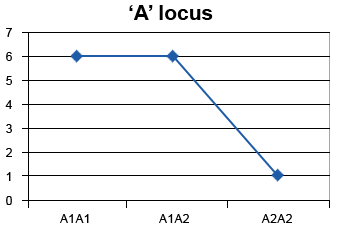
Figure 5 describes dominance effects by showing the non-linear regression (with non-common slope) between genotypes to describe non-additive effects (in this case dominance effect).
Will selection for maximum expression always lead to selection of true breeding individuals? [Hint: consider individuals in early generations compared to purelines in a self-pollinating crop]
Hypothetical Example
If we consider a hypothetical example of two gene loci (no linkage), the proportions of F2 genotypes are as shown in Table 10.
| Genotype | Ratio |
|---|---|
| A1A1B1B1 | 1/16 |
| A1A1B1B2 | 2/16 |
| A1A1B2B2 | 1/16 |
| A1A2B1B1 | 2/16 |
| A1A2B1B2 | 4/16 |
| A1A2B2B2 | 2/16 |
| A2A2B1B1 | 1/16 |
| A2A2B1B2 | 2/16 |
| A2A2B2B2 | 1/16 |
Let’s assume genotypic value as:
A1A1 = A1A2 = 4, A2A2 = 0
B1B1 = B1B2 = 3, B2B2 = 0.
Also assume complete dominance at A and B loci. Then, the genotypic values are as shown in Table 11.
| Genotype | Genotypic value |
|---|---|
| A1A1B1B1 | 7 |
| A1A1B1B2 | 7 |
| A1A1B2B2 | 4 |
| A1A2B1B1 | 7 |
| A1A2B1B2 | 7 |
| A1A2B2B2 | 4 |
| A2A2B1B1 | 3 |
| A2A2B1B2 | 3 |
| A2A2B2B2 | 0 |
Proportions
If a breeder makes selections based only on phenotype, she/he will select plants that have the following genotypes (A1A1B1B1, A1A1B1B2, A1A2B1B1, and A1A2B1B2) in the proportions listed below (with the assumption of independent assortment at the A and B loci).
A1A1B1B1 = 1/16 of the total population,
A1A1B1B2 = 2/16 of the total population,
A1A2B1B1 = 2/16 of the total population,
A1A2B1B2 = 4/16 of the total population,
In this case, the breeder is not able to distinguish between homozygous and heterozygous individuals of the four genotypes above as they have similar phenotypes.
Therefore, if a breeder only wanted homozygous dominant (A1A1B1B1) plants and they only used phenotype to make their selection, they will end up selecting 9 out of 16 plants; however, only 1 out of 16 plants should have been selected.
In a self-pollinated species where a cultivar is an inbred line, non-additive gene effects can rarely be fixed, and therefore, selection response is unpredictable when a trait is controlled by genes acting in a non-additive manner. In a cross-pollinated species where hybrid cultivars are used, non-additive gene effects, especially dominance effects, are important.
Types of Interaction
In the example below (Table 7; Fig. 6), we will look at a hypothetical case of two genes controlling plant height to demonstrate epistatic effects (i.e., the interaction of genes at different loci).
Assume that ‘A’ and ‘B’ loci both affect plant height (shown in cm in Table 12).
| B1B1 | B1B2 | B2B2 | |
|---|---|---|---|
| A1A1 | 90 | 105 | 110 |
| A1A2 | 90 | 95 | 102 |
| A2A2 | 90 | 94 | 95 |
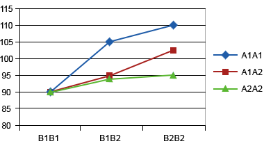
Epistatic interactions can be additive*additive, dominance*dominance or additive*dominance, or a higher order for three loci or more. These interactions are important for most traits as these interactions are common.
Concept of Variability
Johannsen Experiment
If you received a seed lot that had variable seed size, you can select for small and large seed types and grow these seed as individual plants. Each individual plant can be harvested separately and a unique ID given to each row of plants of these individual plants. If you grew each row and measured seed size, what will you expect to find among and within lines in the progeny generation if the original seed lot consisted of a homogenous mixture of purelines (true breeding = homozygous)?
Johanssen, in 1903, conducted an experiment in beans (Phaseolus vulgaris), a highly self-pollinated species, to study the effect of selection for seed weight using a seed lot from the cultivar ‘Princess’. His experiments showed that: a) selection for seed weight was effective in the original unselected population (i.e., lines selected for differences in seed weight showed consistent differences in seed weight in subsequent generations; large seeded parents produced large seeded progeny and small seeded parents produced small seeded progeny), and b) selection within a line was not effective (i.e., irrespective of whether the parent was small or large seeded, all of the progeny of the selected seed always showed the average seed weight typical of the parent line).
Johanssen concluded from this experiment that the original seed lot was composed of a mixture of different genotypes/purelines (that were each homozygous for genes controlling seed weight), and even when the progeny of a seed lot differed phenotypically, each seed of that line possessed the same genotype for seed weight.
Mathematical Representations
Mathematically, the phenotypic value for an individual (i.e., a single seed in Johanssen’s experiment) in a population is equal to its genotypic value plus an environmental (non-genetic) deviation:
[latex]\Large P=G+E[/latex]
where:
P = phenotype (observed seed weight)
G = genotype (genetic potential for seed weight)
E = environment (environmental effects, i.e., factors determining the extent to which genetic potential is reached)
For a population of seed, the phenotypic variability is represented mathematically by the equation below:
[latex]\Large V_P=V_G+V_E[/latex]
where:
VP = phenotypic variability (total variability observed)
VG = genotypic variability (variability due to genetic cause)
VE = environmental variability (variability due to environmental causes)
Genetic variability is heritable, i.e., variability that can be manipulated by plant breeders and transmitted to progeny. The presence of genetic variability (as we saw earlier) is ESSENTIAL for selection to be effective.
Environmental variability is not heritable and it can mask the true expression of a trait.
Phenotype Interactions
If we assume that the mean value of “E” for all individuals across the population is zero, then the mean phenotypic value equals the mean genotypic value. Thus, the population mean is both the phenotypic and genotypic value. To prove this, consider a theoretical experiment using replicated genotypes – either as clones or as inbred lines – and measure them under “normal” environmental conditions. The mean “E” will be zero across the population, so that the mean phenotypic value would equal the mean genotypic value.
However, in reality, plant breeders deal with segregating populations that are not genetically uniform when they are selecting. So let’s explore the types of gene actions and their importance to breeding.
Phenotype, Genotype, Environment, and Genotype X Environment Interactions
Phenotype is governed by Genotype ([latex]σ_G^2[/latex]), and Genotype × Environment interactions ([latex]σ_{GE}^2[/latex]). Not all variation for a phenotype is accounted for by Genotype and GxE interaction with the remaining variation attributed to error. Any trait that you observe for a plant, a plant family, or population is a phenotype. Genotype is the genetic basis of a trait (e.g., gene or gene × gene interactions). GxE interaction is the interaction of genotype with environment, where each genotype may perform or look different in different environments. The environment of a single plant consists of all things other than the genotype of the individual.
The environment includes differences in soil, temperature, humidity, rainfall, day length, solar radiation, wind, salinity, pathogens, pests, etc.
Environment
Environment can be micro-environment or macro-environment. A micro-environment refers to a unique set of factors that alter the development of a single plant. Groups of plants growing at the same time in the same space each encountering similar micro-environment are classed under experiencing a macro-environment (i.e. a class of micro-environments). For example, if a field of beans is exposed to excessive moisture stress (i.e., water logging), individual plants may suffer slightly different levels of water logging (micro-envirionment), but all plants would suffer some degree of water logging (macro-environment). This beans field’s macro-environment will be described as water logged. In breeding, we are more interested in the macro-environments and these are classified as location or year, or a combination of location x year, or simply environment.
To describe the phenotypic value of a genotype in terms of microenvironment and macro-environment, let’s consider the equation below:
[latex]\large P_{ijk} = G_i + E_k + (G*E)_{ik} + e_{ijk}[/latex]
where:
[latex]G_i[/latex]= effect of the [latex]i[/latex]th genotype
[latex]E_k[/latex]= effect of the [latex]k[/latex]th macro-environment
[latex](G * E)_{ik}[/latex]= effect of interaction between [latex]i[/latex]th genotype and [latex]k[/latex]th macro-environment
[latex]e_{ijk}[/latex]= residual composed of deviation of the [latex]j[/latex]th micro-environment from the mean of such effects in the macro-environment [latex]k[/latex], and deviation of the interaction from the mean of interactions.
Graphical Representations of GxE Interaction
Assume two genotypes are tested at two locations. On the y-axis, we present yield/ha, and the x-axis is environment (i.e., locations). Figs. 7, 8, and 9 show different types of GxE interaction:
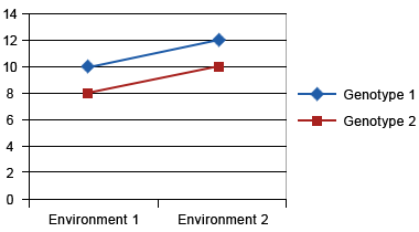
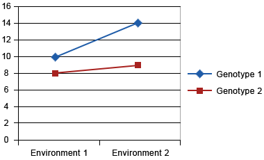
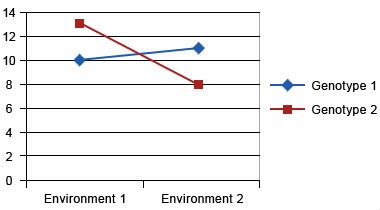
Crossover Interaction
Crossover interaction is the most important type of genotype x environment interaction because different genotypes will be selected in different environments. Crossover interactions are often due to differences in how genotypes respond to different environments. For example in Figure 6, let’s consider that environment 1 is disease free, while pathogen ‘A’ is present in environment 2. Genotype 2 is a high yielding, disease susceptible genotype and genotype 1 is a lower yielding, disease resistant genotype. Genotype 2 will yield higher in environment 1, while genotype 1 will yield higher in disease prevalent environment 2. The goal of a breeder should be to combine the better response to both environments into a single genotype. However, a breeder needs to first determine if yield and disease resistance are mutually exclusive. For example, it’s possible that the gene for disease resistance could be linked to gene(s) that reduce yield. In this case, a breeder would need to grow a large segregating population to identify progeny with useful recombination that combines high yield and disease resistance. If however, a single pleiotropic gene controls both disease resistance and yield, a breeder can only improve both traits by complementation (i.e., the building or bringing together of other useful genes to improve the responses).
Practical Considerations of GxE Interaction for Plant Breeders
- Breeders working at international institutions (CGIAR institutes such as CIMMYT, ICARDA, IRRI, and CIAT) have a mandate of a wider adaptation, while a provincial or state breeding institute’s mandate will be more localized (specific area, perhaps one macro-environment). CGIAR breeders often utilize many (more than 20) diverse locations to identify cultivars with wider adaptation, while breeders at a state breeding institute use fewer environments that are representative of one or two macro-environments.
- If the mandate of the program is to develop cultivars for specific purposes (i.e., disease resistance, stress tolerance, or quality traits), then the testing sites need to be selected by breeders for this objective. For example, malt barley has a very specific crop quality requirement. Stable performance on quality (malt quality for consistent and high quality and better taste for beer-making) is a must and breeders will discard cultivars if they show specific adaptation for malt quality, i.e., only very specific sites produce good malt.
- Resource allocation: A breeder should be aware of the relative importance (i.e., magnitude) of G × Location, G × Year, and G × Location × Year interactions in order to appropriately allocate resources for cultivar testing. This information will help a breeder decide on how many locations and years should be used for testing materials.
- While we have not discussed different stability analysis methods, these methods (such as AMMI type analysis) will help to determine which environments are more similar to each other. Each mega-environment will consist of several individual locations or sites. Within a mega-environment, the genotypes perform more similarly compared to genotypes in different mega-environments. In other words there is little or no G×E interaction among environments within a mega-environment. In such a scenario, breeders will gain little by testing in more similar environments, and should aim to test across dissimilar environments to test for stable performance of genotypes in a range of environments. Breeders should therefore aim to sample one or more locations from each mega-environment (or testing zone). Environmental parameters such as rainfall, soil type, pH, etc., may also be a good way to cluster environments. If there are larger agro-ecological regions that grow predominantly a single cultivar and you as a breeder are targeting for that region, the cultivar acreage map may also serve as a good source to identify mega-environments to develop a better yielding alternative to that large acreage cultivar. Another useful exercise is to perform genetic correlations (genotype means analysis) to see if the correlations are high or low. High correlation will mean that predictive ability of those environments is similar and a breeder does not gain as much information on stability as he/she would gain by testing in environments with lower correlation among genotype means.
- If G×E cannot be measured (due to lack of resources to have more than one site), a breeder should still consider putting that test in two dissimilar conditions, for example dryland versus irrigated nurseries.
Selecting a Testing Site
The site where you grow your trials may have seasonal patterns, such as cycles of drought at seedling stage, heat stress at flowering stage, and years with no apparent stress. It is advisable to keep track of this information (through the use of long term checks that have known and consistent response to these stresses and weather parameters) and use this site for selection to improve tolerance for these factors. If you are breeding for another trait, say salinity tolerance, a new site more appropriate for screening of this trait will be required.
Factors to consider in the selection of testing site include the following:
- Good correlation with the performance in farmer growing conditions.
- Ability to handle different tests (infrastructure) and ability to respond to mitigate threats (such as an ability to irrigate if needed to avoid impact of water deficit on response to the selected treatment).
- Low environmental error, i.e., higher heritability to differentiate ‘keeps’ (i.e., desirables) from discards.
- Infrastructure to implement breeding decisions of timely planting, maintenance, harvest, processing etc.
Adaptation Factors
As we previously covered, the debate on wide versus specific adaptation is still ongoing among breeders and really boils down to:
- the mandate of the program
- target region, and
- farmers.
Ultimately, breeders need to remember that their job is to ensure that the product (cultivar) that reaches farmers can help them to make a profit, and that it meets the requirement of end-user (e.g. the processing industry) who buys from farmers.
If you, a breeder, produce the highest yielding cultivar but it lacks the necessary quality or protection against biotic or abiotic stress, farmers will not grow this variety. Therefore, always think of the cultivar you develop as a “package”. A package needs to have all the ingredients that will make it ready to be adopted by farmers as well as the processing industry.
Heritability
Concept
Definition: Heritability can be defined as the degree to which the characteristics of a plant are repeated in its progeny. Mathematically, we have seen already that it is the proportion of total variability for a character due to genetic causes.
Further theoretical information can be obtained here.
Broad sense heritability: [latex]\large(h^2_b) = \largeσ^2_G/σ^2_P[/latex]
Narrow sense heritability: [latex]\large(h^2) = \largeσ^2_a/σ^2_P[/latex]
where:
[latex]σ^2_G[/latex] is total genotypic variance
and
[latex]σ^2_a[/latex] is the additive component of the genotypic variance.
Narrow sense heritability is more valuable since it indicates how much of the total observed variability is due to additive gene action (which can be selected for effectively and fixed in homozygous condition).
Broad sense heritability is less valuable since it also includes dominance and epistasis (these gene actions cannot be fixed and occur only in specific gene combinations).
Importance
It is important for breeders to have a sense of the heritability of traits that they are selecting for in their programs. This can be obtained by using data from their own experiments, or for a new program, using information available in literature or from previous experiments. The reason heritability is important is that selection response is related to heritability. The higher the heritability, the more the phenotype reflects the genotype and the more effective selection will be. More extensive testing (more environments, more replications) reduces the phenotypic variance and increases heritability. Heritability can be increased more by using higher number of locations rather than by increasing the number of years [this is due to smaller variance component of Genotype × Year, relative to other component such as Genotype × Location]. This suggests that in most cases, a breeder does not need to do selection based on more than one year of data [except in cases where selections are made in each generation as plants are achieving ‘true breeding’ status].
Methods for Estimating Heritability
- Variance Component method: Comparison of segregating and homogenous populations is applicable to only self-pollinated or clonally propagated species. This method estimates broad sense heritability. This method involves estimating the magnitude of various types of genetic and environmental variability.
In such experiments, [latex]σ^2_{P1}=σ^2_{P2}=σ^2_{F1}=σ^2_{E}[/latex]
In a self-pollinated species, parent 1 and parent 2 being inbred, their estimates of genetic variability will be similar to each other ([latex]σ^2_{P1}=σ^2_{P2}[/latex]) as well as to F1 ( [latex]=σ^2_{F1}[/latex]), and these will be equal to environmental variability (as these three are genetically uniform and therefore any variability observed will be due to environment). Variance of F2 or any other segregating generation can then be used to obtain [latex]σ^2_{P}-σ^2_{E}[/latex]), where [latex]σ^2_{P}[/latex] is variance estimated from the segregating generations. - Covariance between relatives (or resemblance among relatives as measured by regression analysis): Examples are, parent-offspring regression, covariance between half-sibs and full-sibs, covariance between inbred or partially inbred families. Variability estimates can be obtained in other ways such as special mating designs (half-sib, full-sib, North Carolina designs, etc.), or analysis of trials conducted in a range of environments.
- Realized heritability [see Response to Selection section, below]
Example 1
Table 13 is an example of analysis of variance (ANOVA) where a random set of genotypes were evaluated over ‘[latex]l[/latex]’ locations for ‘[latex]y[/latex]’ years, and ‘[latex]r[/latex]’ replications used in each test. Multiple locations, years and reps.
| Source of variation | Degrees of freedom | Mean square | Expected mean square |
|---|---|---|---|
| Location ([latex]L[/latex]) |
[latex](l-1)[/latex] | n/a | [latex]\sigma ^2_{e} + r\sigma ^2_{gly} + ry\sigma ^2_{gl} + g\sigma ^2_r + gr\sigma ^2_{ly} + gry\sigma ^2_l[/latex] |
| Year ([latex]Y[/latex]) |
[latex](y-1)[/latex] | n/a | [latex]\sigma ^2_{e} +r\sigma ^2_{gly} +ry\sigma ^2_{gl} +g\sigma ^2_{r} +gr\sigma ^2_{ly} +grl\sigma ^2_{y}[/latex] |
| [latex]L*Y[/latex] | [latex](l-1)(y-1)[/latex] | n/a | [latex]\sigma ^2_{e}+r\sigma ^2_{gly}+ry\sigma ^2_{gl}+g\sigma ^2_{r}+gr\sigma ^2_{ly}[/latex] |
| Rep ([latex]L*Y[/latex]) |
[latex]ly(r-1)[/latex] | n/a | [latex]\sigma ^2_{e}+g\sigma ^2_{r}[/latex] |
| Genotype ([latex]G[/latex]) |
[latex](g-1)[/latex] | [latex]MS_1[/latex] | [latex]\sigma ^2_{e}+r\sigma ^2_{gly}+ry\sigma ^2_{gl}+rl\sigma ^2_{gy}+rly\sigma ^2_{g}[/latex] |
| [latex]G*L[/latex] | [latex](g-1)(l-1)[/latex] | [latex]MS_2[/latex] | [latex]\sigma ^2_{e}+r\sigma ^2_{gly}+ry\sigma ^2_{gl}[/latex] |
| [latex]G*Y[/latex] | [latex](g -1)(y -1)[/latex] | [latex]MS_3[/latex] | [latex]\sigma ^2_{e}+r\sigma ^2_{gly}+rl\sigma ^2_{gy}[/latex] |
| [latex]G*L*Y[/latex] | [latex](g-1)(l-1)(y-1)[/latex] | [latex]MS_4[/latex] | [latex]\sigma ^2_{e}+r\sigma ^2_{gly}[/latex] |
| Pooler Error | [latex]ly(g-1)(r-1)[/latex] | [latex]MS_5[/latex] | [latex]\sigma ^2_{e}[/latex] |
where:
[latex]σ^2_{e}=MS_5[/latex]
[latex]σ^2_{gly} = (MS_4 = MS_5)/r[/latex]
[latex]σ^2_{gy}=(MS_3-MS_4)/rl[/latex]
[latex]σ^2_{gl}=(MS_2-MS_4)/ry[/latex]
[latex]σ^2_{g}=(MS_1-MS_2-MS_3+MS_4)/rly[/latex]
[latex]σ^2_{P}[/latex] (phenotypic variance of genotypic means) = [latex]σ^2_{g}+\frac{σ^2_{gl}}{l}+\frac{σ^2_{gy}}{y}+\frac{σ^2_{gly}}{ly}+\frac{σ^2_{e}}{rly}[/latex]
and if we substitute for Mean squares we will obtain,
[latex]σ^2_p =\dfrac {MS_1}{rly}[/latex]
Broad Sense heritability can be calculated using the equations above.
Example 2
Table 14 is an example of analysis of variance (ANOVA) where a random set of genotypes were evaluated over ‘[latex]e[/latex]’
environments (can be locations, years or combination of years and locations), and ‘[latex]r[/latex]’ replications used in each test. Multiple environments and reps within a year.
| Source of variation | Degrees of freedom | Mean square | Expected mean square |
|---|---|---|---|
| Environment ([latex]E[/latex]) | [latex](e-1)[/latex] | n/a | [latex]σ^2_{e}+gσ^2_{r(e)}+rσ^2_{ge}+rgσ^2_{e}[/latex] |
| Rep ([latex]E[/latex]) | [latex]e(r-1)[/latex] | n/a | [latex]σ^2_{e}+gσ^2_{r(e)}[/latex] |
| Genotype ([latex]G[/latex]) | [latex](g -1)[/latex] | MS1 | [latex]σ^2_{e}+rσ^2_{ge}+reσ^2_{g}[/latex] |
| [latex]G*E[/latex] | [latex](g-1)(e-1)[/latex] | MS2 | [latex]σ^2_{e}+rσ^2_{ge}[/latex] |
| Pooler Error | [latex]e(g-1)(r-1)[/latex] | MS3 | [latex]σ^2_{e}[/latex] |
Note: all factors considered random in ANOVA.
[latex]σ^2_{e}=MS_3[/latex]
[latex]σ^2_{ge}=(MS_2-MS_3)/r[/latex]
[latex]σ^2_{g}=(MS_1-MS_2)/re[/latex]
Variables
[latex]σ^2_p[/latex] (phenotypic variance of genotypic means) = [latex]σ^2_g+(σ^2_{ge})/e+(σ^2_{e})/re[/latex],
If we substitute for Mean squares we will obtain, [latex]σ^2_p = (MS_1)/re[/latex]
Total phenotypic variance [latex]σ^2_p=σ^2_{g}+σ^2_{ge}+σ^2_{e}[/latex]
Heritability on individual experimental unit basis is: [latex]\dfrac{σ^2_{g}}{(σ^2_{g}+σ^2_{ge}+σ^2_{e})}[/latex]
Heritability on genotypic mean basis is: [latex]\dfrac{σ^2_{g}}{(σ^2_{g}+(σ^2_{ge})/e+(σ^2_{e})/re)}[/latex]
This estimate of heritability is obtained if the genotypes represent the population and are chosen randomly. If the genotypes are not chosen randomly (e.g. selected genotypes), the ratio between genetic and phenotypic variation is called repeatability and this estimate is a measure of the precision of data and a measure of the proportion of genetic variation, which helps breeders to detect significant difference among genotypes.
Summary
Each heritability estimate is unique and reflective of the method of calculation, testing environment, generation used in estimation, and genotypes studied. While the heritability estimates are going to somewhat differ based on different conditions described above, a plant breeder can get a good handle on heritability based on published literature, and their or their predecessors’ experiences working on the crop and for various traits.
Heritability is used to estimate the expected response to selection and to choose the best breeding approach to improve the target trait(s). Traits with high heritability can be selected on a single-plant basis in an early generation and in fewer (even single) environments.
A breeder should consider a range of heritability (rather than absolute value) as well as have some precision around their estimate (confidence interval). Higher heritability, say, 0.7, or higher narrow sense heritability means a breeder can expect that selection in early generation can be effective for that trait. High broad-sense heritability only indicates that effect of environment is smaller but does not provide insight into the relative importance of additive (which can be fixed) or non-additive (which cannot be fixed) gene effects.
Selection Theory
Truncation
When individuals are selected based on their individual phenotypic value, we call this artificial selection or individual selection. Truncation is a type of individual selection and very common in plant breeding programs. The curve in Figure 10a represents the normal distribution of a quantitative trait in a population, and the shaded part ‘T’ (i.e., truncation point) represents the individuals selected for the next generation of breeding – could be cross- or self-pollinated. µ is the mean of the unselected population (or mean of the population in generation 1) and µs is the mean of selected parents. If these selected parents are mated at random, their offspring will have the phenotypic distribution in Figure 10b and a mean equal to µ‘. Generally, µs > µ’ > µ.
- µ’ is greater than µ because some of the selected parents have favorable genotypes and therefore pass favorable genes on to their offspring.
- µs is greater than µ’ because some of the selected parents did not have favorable genotypes, but instead had superior phenotype due to the favorable environment where they were tested (chance exposure to favorable environment, e.g., low spot in the field that received more water, a spot in the field that received more fertilizer, or a spot in the field that was not exposed to high winds). Secondly, alleles, not genotypes, are transmitted to the offspring and favorable genotypes may segregate or recombination may cause breakage of favorable linkages.
Equations
The difference in mean phenotype between the selected parents ([latex]µ_s[/latex])
and generation 0 ([latex]µ[/latex])
is called selection differential ([latex]S[/latex]).
[latex]\Large {S}=\mu _{\small S}-\mu[/latex]
Equation 1
The difference in mean phenotype between the progeny generation (generation 1) ([latex]µ’[/latex])
and generation 0 ([latex]µ[/latex])
is called the response to selection ([latex]R[/latex]).
[latex]\Large {R}=\mu' - \mu[/latex]
Equation 2
The prediction equation defines the relationship between [latex]S[/latex]
and [latex]R[/latex]. For truncation selection, the prediction equation is:
[latex]\Large {R}={h}^{2}* {S}[/latex]
Equation 3
where, [latex]h^2[/latex] is heritability of the trait.
Graphical Representation
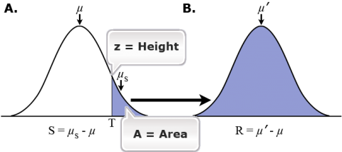
A. phenotype distribution in parental population with mean [latex]\mu[/latex]. Shaded area shows the individuals that were advanced to the next generation (individuals with phenotypes above the truncation point ( [latex]T[/latex]). Selected individuals (shaded area) have a meaning phenotype ([latex]\mu_S[/latex]).
B. distribution of phenotypes in offspring generation derived from the selected parents. the mean phenotype is donated with ([latex]\mu'[/latex]). [latex]S[/latex] = selection differential, [latex]R[/latex] = response to selection. Source: Harti, D. (1988). Primer of Population Genetics, 2nd edition. Sinauer Association.
z/A = frequency at the truncation point (in a normal distribution)/Area under the selected portion of the curve. This is equal to selection differential/phenotypic variance, i.e.,
[latex]\large {z}/{A}=\left ( \mu -\mu ' \right )/\sigma ^{2}[/latex]
Equation 4
assuming that the effects of each allele are small relative to phenotypic variation, and phenotypic values are normally distributed.
Response to Selection
Calculations
We cannot get into detailed calculation, but it can be shown that:
[latex]\mu' = \mu + 2 \Big[a+(q-p)d \Big] \Delta p[/latex]
Equation 5
where:
[latex]\Delta p = \text{change in allele frequency of A1} = (z/A)*pq \Big[a+(q-p)d \Big][/latex]
[latex]a[/latex] = genotypic effect
[latex]d[/latex] = measure of dominance
[latex]p[/latex] = allele frequency of A1
[latex]q[/latex] = allele frequency of A2
[latex]\mu'[/latex] = mean phenotype of progeny generation
[latex]\mu[/latex] = progenitor generation
Substituting z/A = (µs – µ)/ σ2p and Δp, equation can be written as:\
[latex]\mu-\mu' = \Big\{ ( \mu_{s}-\mu ) \times \textrm{2pq} \times[\textrm{a}+ ( \textrm{q-p} )\textrm{d} ]^{2} \Big\} / \sigma_\textrm{p}^{2}[/latex]
Equation 6
Since, S = µs – µ and R = µ’ – µ,
[latex]\textrm R = \Big\{ \textrm S \times \textrm{2pq} \times[\textrm{a}+ ( \textrm{q-p} )\textrm{d} ]^{2} \Big\} / \sigma_\textrm{p}^{2}[/latex]
Equation 7
Additive Genetic Variation
We already have seen that R = h2S (Equation 3), therefore, we can now define heritability in the genetic terms of: a, p, q, d, σ2p as:
[latex]\textrm h^2 = \Big\{\textrm{2pq} \times[\textrm{a}+ ( \textrm{q-p} )\textrm{d} ]^{2} \Big\} / \sigma_\textrm{p}^{2}[/latex]
Equation 8
This heritability definition is valid when the trait is under single gene control. This is hardly the case for most of the traits, therefore heritability (narrow sense) can be defined as:
[latex]\textrm h^2 = \Big\{\sum \textrm{2pq} \times[\textrm{a}+ ( \textrm{q-p} )\textrm{d} ]^{2} \Big\} / \sigma_\textrm{p}^{2}[/latex]
Equation 9
Σ2pq[a + (q – p)d]2 = additive genetic variation of the trait = σ2a
Selection Intensity
Selection Intensity and Response to Selection Equation
R = h2S can also be written as:
[latex]\LARGE {R}={i}\sigma {h}^{2}[/latex]
Equation 10
[latex]\LARGE {S}={i}\sigma =\sigma ^{2}{z}/{A}[/latex]
Equation 11
where:
[latex]i[/latex] = standardized selection differential.
Intensity of selection depends on the proportion of the total population selected. For example, Table 15 shows some selection intensities based on % selected (assuming a completely normal trait distribution). The full table can be seen in most plant breeding books.
| % selected | Standardized selection differential (i) |
|---|---|
| 0.01 | 3.959 |
| 0.1 | 3.367 |
| 0.5 | 2.892 |
| 1 | 2.665 |
| 5 | 2.063 |
| 10 | 1.755 |
| 15 | 1.554 |
| 20 | 1.400 |
| 25 | 1.271 |
| 30 | 1.159 |
| 35 | 1.058 |
| 40 | 0.966 |
| 45 | 0.880 |
| 50 | 0.798 |
h2 is narrow sense heritability
σp = phenotypic standard deviation (=square root of phenotypic variance)
Breeder’s Equation
This equation R = iσh2 (Equation 10) is fundamental in plant breeding. Plant breeders generally do not use it to calculate an actual numerical value for selection response. However, this equation is important as it shows that selection response depends on:
- Selection intensity
- Heritability
- Phenotypic variability present in the population, say from a cross.
The equation R = µ’ – µ can be written as
[latex]\Large \mu '=\mu +{i}\sigma {h}^{2}[/latex]
Equation 12
which clearly indicates that to maximize the expression of a trait in the offspring generation, a breeder needs to start with high expression of the trait, maximum heritability, and high selection intensity (although diminishing returns apply beyond a certain level).
Square root of heritability (h) is a measure of the correlation between the observed phenotypic value and the underlying genotypic value. In a breeding program, a breeder will try to maximize these factors (higher standardized selection differential, genetic variation, heritability). One has to keep in mind that optimum balance needs to be obtained between increased expected response (which is a good thing and what a breeder is after) and increased variability of that response (undesirable characteristics of selection). We will look at a few examples below to understand the concept of variability of response.
[latex](C.V.\ of\ R) = \sqrt{\frac{\large1+(p\,\times\,h^2)-(h-h^2)}{\large p\,\times\,n\,\times\,i\,\times\,i\,\times\,h^2\,\times\,h^2}}[/latex]
Equation 13 (From Baker, 1971.)
where:
n = total number of lines evaluated
p = proportion of lines selected
h2 = heritability
i = standardized selection differential
C.V. = coefficient of variation
For example, assume a breeder started with n=1000, % selected (p) = 0.01, heritability (h2) = 0.2, and i = 3.959, then CV (Response to selection) = 39% by substituting values in Equation 10.
n = total number of lines evaluated = 1000
p = proportion of lines selected = 0.01
h2 = heritability = 0.2
i = standardized selection differential = 3.959
C.V. (R) = 30%
Compared to starting with a smaller number of lines, if a breeder started with n=100, % selected = 0.01, heritability = 0.2, and i = 3.959; CV (Response to selection) = 124%.
n = total number of lines evaluated = 100
p = proportion of lines selected = 0.01
h2 = heritability = 0.2
i = standardized selection differential = 3.959
C.V. (R) = 124%
Importance of h-squared
However, h2 importance can be seen with the same calculations: if a breeder started with n=1000, % selected = 0.01, heritability = 0.7, and i = 3.959; CV (Response to selection) = 8%.
n = total number of lines evaluated = 1000
p = proportion of lines selected = 0.01
h2 = heritability = 0.7
i = standardized selection differential = 3.959
C.V. (R) = 8%
If breeder had started with n=1000, % selected = 5, heritability = 0.7, and i = 2.063; CV (Response to selection) = 2%.
n = total number of lines evaluated = 100
p = proportion of lines selected = 5
h2 = heritability = 7
i = standardized selection differential = 2.063
C.V. (R) = 2%
These calculations show that while the response to selection equation is an essential equation for any breeder to consider for trait improvement, it is also worthwhile to consider the extent of variability in relation to the mean of the population (CV).
Selection Explanation
One of the ways to maximize genetic standard deviation is to cross diverse parents. However, if crosses between diverse parents have lower unselected means than crosses between adapted (elite) parents (which will have lower genetic variability between them, generally), then a breeder may be reducing the mean genotypic value of the subsequent population by crossing diverse parents. Therefore, best x best (or elite x elite) crosses is one way to maximize genotypic mean of the starting population although it may reduce the genotypic variance and even response to selection, R. Most cultivar development programs will work with best x best configuration, or have at least 75% elite, for example, (best x exotic) x best.
Standardized selection differential can be increased by selecting fewer lines (but we saw earlier that this can cause increased variability of response, which is undesirable) or testing more units but selecting fewer units (this will require more resources). If a breeder makes compromises between testing more lines to advance a few, it will likely be done at a compromise of not doing a thorough evaluation of units. Less thorough evaluation will result in lower correlation between phenotypic and genotypic values (lower h), therefore a breeder should not compromise on proper trait measurement protocols. Optimum balance needs to be achieved for each trait for more thorough testing to increase the correlation between phenotypic and genotypic values (higher h) as well as increase the standardized selection differential.
Expected Genetic Gain
Expected genetic gain formula is shown below.
[latex]\LARGE \Delta G = \frac{ic}{y} \frac{\sigma^2_G}{\sqrt{\sigma^2_p}}= \frac{ic}{y} \frac{\sigma^2_G}{\sqrt{\frac{\sigma^2_e}{re}+\frac{\sigma^2 _{GE}}e{+ \sigma^2_G}}}[/latex]
Equation 14
This formula is an extension of response to selection:
[latex]\LARGE R = h^2S = ih^2 \sigma _P = \frac{i \sigma^2_g}{\sqrt{\sigma^2_P}}=\frac{c}{y}=\frac{i\sigma^2_g}{\sqrt{\sigma^2_P}}[/latex]
Equation 15
and includes two additional variables: number of years (y) and parental control (c) (Eberhart, 1970) compared to what we have seen so far.
Heritability equation is
[latex]\Large\dfrac{\sigma^2_g}{(\sigma^2_g \,+ \,(\sigma^2_{ge})/e \, +\,\sigma^2_e)/re)}[/latex]
Equation 16
where:
[latex]r[/latex] =number of replications
[latex]e[/latex] =number of environments
We have already looked at i, which is standardized selection differential, c = parental control, and y = seasons per cycle.
Practical Considerations
- Increase the numerator of this equation by increasing genetic variance (larger population sizes, diverse parents (but keep the proportion of elite parents high), increasing selection intensity (without getting genetic drift problem).
- Parental control will allow for increased response to selection. Parental control, c, can be increased by recombining genotypes where both sources of gametes originated in selected genotypes (c = 1), which will be generally true in self-pollinated crops. In cross-pollinated species, c = 0.5 if the male gametes are coming from unselected genotypes. Therefore, it is recommended that if possible, conduct selection before pollination so that only selected genotypes contribute to the next generation. C = 2.0 if the selected seed of selected genotypes is used for establishing the next generation.
- Another way to increase genetic gain is to decrease the value of the denominator. This can be achieved by decreasing the number of seasons per cycle or the phenotypic variance (which can be decreased by reducing g x e and e variances. The phenotypic variance can be decreased by increasing the number of locations (or environments) and by increasing replication. Increasing locations is generally considered to play a more important role in reducing phenotypic variance rather than replications.
- Usage of proper experimental methods and field design and analysis will reduce error variance and improve confidence in estimate of progeny performance. These methods may include augmented designs, or moving means in earlier generations where no replication is used per environment and using incomplete lattice (for example, alpha-lattice) or RCBD in replicated tests.
- Different generations and type of progenies have different genetic variance components and therefore affect the equation. The theoretical proportion of additive variance to total genotypic variance of half sib is 0.25, full-sib is 0.5 and 1 for S1 progenies.
- The number of seasons required to complete a cycle can be reduced by using off-season nurseries, or by using an off-season nursery with high correlation to the home environment to facilitate selection for high to moderate heritability traits and to reduce the ‘y’ in equation above. If resources permit, greenhouse or growth cabinet can be used instead of off-season nursery and complemented with marker assisted selection to increase ‘i’ as well as reduce ‘y’.
Reducing Effect of Environment
One way to obtain higher heritability is to reduce environmental effects (remember, higher heritability implies that selection will be more effective as ‘what you see is what you will get’).
Here are some recommendations to reduce the effect of environment:
- Use best quality land (uniform area – less gradients in field, highly productive) if selection will be performed (on single plant, rows, or yield trials; in early or later generations).
- Use best management practices (reflective of the recommended fertilizer, irrigation, crop rotation, time of planting, weeding, harvesting). An advice is to avoid pest or pathogen control as this will provide another trait to select for if naturally present].
- Use check cultivars frequently (this will allow breeders to have a better handle on variability).
- Use appropriate statistical designs (lattice, RCBD, augmented designs as needed).
- Use replication (improves precision, and provides better handle to measure variation) and randomization (improves accuracy).
Multiple Trait Selection
- Tandem selection: A breeder selects sequentially for each trait in successive generations. In this scenario, population is improved first for one trait, then for the next trait and so on. This will lead to improvement over generations. One disadvantage of this strategy is long selection cycle, and is generally not followed in commercial plant breeding. Another disadvantage of this strategy is the potential reduction in the level of performance of the first trait selected.
- Independent culling (or truncation selection): Selection is practiced successively in the same generation. This is probably the most common selection strategy deployed by breeders worldwide. In this scheme, a breeder will discard all individuals that fail to meet the desired level for one trait, irrespective of the value for any of the other traits. This will be followed by selecting among the surviving lines for the second trait and the process is repeated until all selections are made. Experienced breeders will know the culling point keeping in mind the trait value of the most important trait, and may allow some relaxation for major traits when culling for traits that have less significance or importance. One issue with independent culling is that with each successive trait cull, the population size and genetic variability is reduced.
- Index selection: An index is developed based on the combination of the heritability and economic value of each of several traits under selection, simultaneous selection is happening for every trait in the same generation. Each line is given an index score based on the trait expression and weight given to the trait. Most breeders use a “mental” index selection. For example, visual selection may be done for a number of traits, an overall mental assessment done, and selection is made. For example, in a space planted nursery where single plants are growing, a breeder may make a mental assessment on the criteria for different traits such as height, seed fill, plant health, lodging, inflorescence and either keep or discard. Since there are likely several thousand plants in a nursery, “mental” index approach needs to be used, as the most feasible. There are more sophisticated methods described such as Pesek baker index (Pesek and Baker, 1969) but these require estimation of variance and co-variances. Using economic weights is a good compromise to remove the need to know variance and co-variances. However, it is still not an easy task to develop an index.
Combining Ability
GCA and SCA
Combining ability of inbred lines is of paramount importance in determining future usefulness and commercial potential of the inbred lines for hybrid production. Combining ability can be divided into general combining ability (GCA) and specific combining ability (SCA) (Sprague and Tatum, 1942). This concept has been very important in the commercial success of maize breeding and hybrid development.
GCA is defined in terms of the average performance of a line in hybrid combinations. The GCA is calculated as the average of all F1s having this particular line as one parent, the value being expressed as a deviation from the overall mean of crosses.
SCA is defined in terms of instances in which performance of certain hybrid combinations (between two inbred lines in a single cross) is either better or poorer than would be expected based on the average performance of the parent inbred lines. That is, each cross has an expected value that is the sum of GCAs of its two parental lines. However, each cross may deviate from the expected value to a greater or lesser extent, and the deviation is referred to as the specific combining ability (SCA) of the two lines in combination. Estimates of GCA and SCA are applicable to the particular set that a breeder has used in the crossing. These crossings are generally in a diallel design (full or partial, or other designs such as NC designs). Sprague and Tatum (1942) reported that for unselected inbred lines, GCA was relatively more important than SCA, whereas for previously selected lines SCA was more important than GCA. GCA is an indication of genes having largely additive effects (differences of GCA are due to the additive and additive × additive interactions in the base population) and therefore more important in a population such as synthetics, while SCA is indicative of genes having dominance and epistatic effects (differences in SCA are attributable to non-additive genetic variance) therefore more important in a hybrid combination.
Calculations
NOTE: GCA is the average performance of a plant in a cross with different tester lines, while the SCA measures the performance of a plant in a specific combination in comparison with other cross combinations.
Let us look at some calculations:
As we previously described, deviation of the parent mean (X) from the mean of all crosses or population mean (μ) is the general combining ability, therefore we can calculate GCA as:
[latex]\Large GCA = X - \mu[/latex]
GCA of a parent A can be defined as
[latex]\Large Y_i = \mu + GCA_A + e_i[/latex]
Example
Below is an example to show GCA calculation using an experiment where eight inbreds were mated to produce 16 crosses. Response variable was grain yield.
| Cross mean | E | F | G | H | Half-sib mean |
|---|---|---|---|---|---|
| A | 91 | 92 | 77 | 84 | 86 |
| B | 83 | 86 | 75 | 120 | 91 |
| C | 82 | 98 | 85 | 103 | 92 |
| D | 104 | 112 | 87 | 101 | 101 |
| Half-sib mean | 90 | 97 | 81 | 102 | 92.5 |
GCAA -6.5 (=86 – 92.5)
GCAB -1.5
GCAC -0.5
GCAD 8.5
GCAE -2.5
GCAF 4.5
GCAG -11.5
GCAH 9.5
SCAAE = 3 (i.e., full-sib mean – (mid-parent value)) or [91 – (86+90)/2]
SCAAF = 0.5
Etc.
Diallel Example
In the case of a diallel, the calculations of GCA are shown in Table 17 below.
| Cross mean | B | C | D | E | Total | GCA | |||
|---|---|---|---|---|---|---|---|---|---|
| A | 91 | 92 | 77 | 84 | 344 (=91+92+77+84) | -7.2 | |||
| B | n/a | 86 | 75 | 120 | 372 (=91 + 86 +75 + 120) | 2.1 | |||
| C | n/a | n/a | 85 | 103 | 366 (=92 + 86 + 85 +103) | 0.1 | |||
| D | n/a | n/a | n/a | 101 | 338 (=77 + 75 + 85 + 101) | -9.2 | |||
| E | n/a | n/a | n/a | n/a | 408 (=84 + 120 + 103 + 101) | 14.1 | |||
| n/a | n/a | n/a | n/a | n/a | 1828 (=344+372+366+408) | n/a | |||
| Note: “n/a” means cell is blank. | |||||||||
Expected value of a cross between inbred lines ‘A’ and ‘B’ is
[latex]\large \textrm{X}_{AB}=\mu+ \textrm{GCA}_{\textrm{A}}+\textrm{GCA}_{\textrm{B}}+\textrm{SCA}_{\textrm{AB}}[/latex]
where:
[latex]μ[/latex] = general mean
and
[latex]\large\textrm{GCA}_{\textrm{A}}=\Big[T_{A}/(\textrm{n}-2)\Big]-\Big[\sum\textrm{T}/\text{n}(\textrm{n}-2)\Big][/latex]
where:
A represents a specific inbred
T = Mean of hybrid performance across each parent for a trait
n = number of parents used in crosses, which is 5 in this case
(From Acquaah, 2007.)
GCAA = [344/(5-2)] – [1828/5(5-2)] = -7.2
GCA for other inbreds can be calculated similarly.
Expected value of the cross between A and B = -7.2 + 2.1 + 91.4 = 86.3
[91.4 = average of all SCA’s]
The SCA is calculated as follows: SCAAB = 91 – 86.3 = 4.7
Heterosis
Heterosis is the superior performance of crosses relative to their parents (Shull 1910; Falconer and Mackay, 1996). Mid-parent heterosis is the difference between the hybrid and the mean of the two parents used in developing the hybrid and can be calculated as
[latex]\large \textrm{Heterosis}_\textrm{(Mid-Parent)}=((\mu_{F1}-\mu_{MP})/\mu_{MP}) \times 100[/latex]
where:
μ = trait mean of the hybrid
μ MP = trait average of the two parents
High-parent heterosis is the superiority of a hybrid over the better parent.
Heterosis is dependent on the presence of dominance and summation of allele frequency differences across loci. In maize and other cross-pollinated crops, heterotic groups have been created such that they maximize the difference in allele frequencies in genes affecting target trait(s) thereby maximizing heterosis.
Examples of hybrid cultivars include: commercial single-cross maize hybrids, commercial three-way cross maize hybrids, and sunflower hybrids. Hybrid cultivars are usually utilized for allogamous species but some hybrids are produced for some autogamous species (i.e., sorghum, tomato, rice). Single-cross hybrid cultivars are homogeneous and heterozygous. Three-way hybrids are both heterogeneous and heterozygous.
References
Baker, R J. 1971. Theoretical variance of response to modified pedigree selection. Can J Plant Sci, 51, 463-468.
Eberhart, S.A. 1970. Factors affecting efficiencies of breeding methods. Afr. Soils. 15:669-680.
Pesek, J., and R.J. Baker. 1969. Desired improvement in relation to selection indices. Can. J. Plant. Sci. 9:803-804.
Shull, G.H. 1910. Hybridization methods in corn breeding. Am. Breed. Mag. 1:98-107.
Sprague, G.F., and L.A. Tatum. 1942. General vs specific combining ability in single crosses of corn. J. American Soc. Agron., 34: 923-932.
