
Chapter 7: Inbreeding and Heterosis
Laura Merrick; Jode Edwards; Thomas Lübberstedt; Arden Campbell; Deborah Muenchrath; Shui-Zhang Fei; William Beavis; and Walter Suza
Introduction
This module focuses on inbreeding, a type of mating of individuals that is often of particular significance to plant breeders. Inbreeding is defined as the mating of individuals that are related by ancestry. Self-pollination (mating of an individual to itself) represents the most extreme form of inbreeding. Inbreeding leads to an increase in homozygosity at the expense of heterozygosity. A key feature of inbreeding is that as homozygosity increases in a population undergoing inbreeding in the absence of selection, the genotype frequency changes while the allele frequency stays unchanged. Inbreeding may occur unintentionally as a result of selection or maintenance of small populations. Inbreeding is also deliberately practiced as a method to create genetic uniformity in populations of interest for genetic or breeding research, for retaining genotypes of inbred cultivars of self-pollinated species through many years of production, or for reliable production of inbred lines to be used in the development of commercial hybrid cultivars.
Inbreeding Depression
A phenomenon known as inbreeding depression—the reduced survival and fertility of offspring of related individuals—occurs in both plants and animals, showing that variation for heritable fitness traits occurs within populations. The occurrence of inbreeding depression varies across species. Charles Darwin, British naturalist famous for his theories of evolution and natural selection was the first person to make a distinction between plants that are outbreeders (species with reproductive mechanisms promoting cross-pollination, who typically exhibit inbreeding depression and tend to be intolerant of inbreeding, e.g., maize and alfalfa) and inbreeders (species with reproductive mechanisms promoting self-pollination in which inbreeding depression is minimal, who tolerate many generations of inbreeding, e.g., wheat and oat). Darwin noticed that:
- outcrossing is more common in nature than self-fertilization
- there are complex reproductive systems that promote outcrossing in plants
- many plant species have evolved systems that prevent self-fertilization.
This module also describes hybrid vigor or heterosis, which is a phenomenon that is functionally the opposite of inbreeding depression. Heterosis is defined as the increased vigor of F1 progeny resulting from the mating of inbred parents. Generally, the performance of the F1 hybrid exceeds the performance of its inbred parents for various traits. The expression of hybrid vigor might affect phenotypes under single gene or polygenic control, e.g., size, growth rate, fertility, and yield. The first-generation offspring of crosses from mating between different pure-line inbreds generally show in a greater amount of desired traits of both parents, but hybrid vigor decreases in F2 and subsequent selfing generations due to inbreeding. The exploitation of hybrid vigor or heterosis is a key feature in the success of hybrid cultivars.
Several mechanisms promote cross-pollination.
- Emergence or maturity of the staminate and pistillate flowers is asynchronous.
- Flowers are monoecious or dioecious.
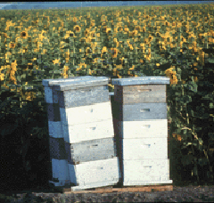
- Mechanical obstruction between the staminate and pistillate flowers in the same individual prevents self-pollination. Alfalfa flowers, for example, have a membrane over the stigma that precludes self-pollination. When a bee lands on the flower, the keel is tripped, rupturing the membrane and exposing the stigma to pollen carried by the bee from other plants it has visited, effecting cross-pollination.
- Gametes produced on the same plant or clone are unable to effect fertilization.
- Self-sterility – gametes from same individual cannot successfully fuse to form a zygote. Sterility can be caused by lack of function of pollen (male gametes) or ovules (female gametes). Male sterility, either genetic or cytoplasmic, occurs because the pollen is not viable. Female sterility occurs when the ovule is defective or seed development is inhibited.
- Self-incompatibility – self-pollination may occur, but fertilization and seed set fail.
Pollen is transported from the staminate flower to the pistillate flower by wind, insects, or animals. Occasionally pollen is transported to receptive stigma of the same individual and self-pollination may occur. For example, pollen from the tassel of a maize plant may land on and pollinate silks on the same plant, effecting self-pollination.
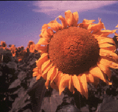
Sunflower is ordinarily cross-pollinated. Bees often carry pollen from one plant and deposit it on other plants.
Several floral mechanisms enforce self-pollination.
- Flowers do not open, preventing external pollen from reaching the stigma.
- Anthesis occurs before the flower opens.
- Stigma elongates through the staminal column (filaments and anthers) immediately after anthesis.
- Floral organs may obscure the stigma after the flower opens.
Although these mechanisms usually enforce self-pollination, a low frequency of cross-pollination may occur. The frequency of cross-pollination in normally self-pollinating species generally depends on the species and environmental conditions.
Soybean is an example of a species that is normally self-pollinated. Before the flower opens, the anthers burst and pollen grains fall out of the anthers on to the receptive stigma contained in the same flower-self-pollination occurs.
Objectives
- Understand the effects of inbreeding.
- Be able to assess the amount of inbreeding by consideration of the inbreeding coefficient.
- Compare and contrast systems of mating that promote inbreeding—self-pollination, half-sib mating, full-sib mating, and backcrossing.
- Learn why inbreeding depression occurs and know why it happens more commonly in species that are predominately cross-pollinated vs. those that are predominately self-pollinated.
- Understand the effects of heterosis and know the difference between the dominance vs. the overdominance hypotheses for explaining its occurrence.
Genetics of Inbreeding
Inbreeding as a Probability
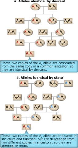
Inbreeding is characterized by a departure from random mating and involves preferential mating between relatives. The most significant effect of inbreeding is that replicates of a single allele in a common ancestor can come together through the mating of relatives to produce homozygous progeny whose alleles are identical by descent. In contrast in a second type of homozygote, two alleles that are said to be alike in state are those that have the same function, but did not derive from replication of a single ancestral gene. These two types of homozygotes can be understood by analyzing pedigrees such as the ones shown in Fig.3. The two copies of the A1 allele in the A1A1 offspring individual at the bottom of Fig. 3a descend from the same copy in a common ancestor; this type of genotype is termed autozygous. In contrast the two copies of the A1 allele in the A1A1 offspring individual at the bottom in Fig. 3b are descended from two different copies in ancestors; this type of genotype is allozygous.
Inbreeding can be estimated directly by studying pedigrees or lineages of ancestry showing genetic relationships.
Measurement of Inbreeding
The probability that two genes are identical by descent is called the coefficient of inbreeding (denoted as F) and will be the measure of relationship between mating pairs.
The coefficient of inbreeding (F) is defined as the probability that two alleles at the same locus are identical by descent. At the population level, F describes the average level of homozygosity. The coefficient of inbreeding is always expressed relative to a specified base population. The base population is defined to be non-inbred (F=0). The range of F is 0 to 1, with 0 indicating random mating and no inbreeding, while 1 means prolonged selfing.
Consider a base population consisting of N individuals each shedding equal numbers of gametes uniting at random (although see Fehr, 1987, p.113, with respect to the concept of effective population size, or Ne). Because the base is defined to have F=0, each individual in this population carries genes that are non-identical. The only way a homozygote that carries genes that are identical by descent can arise is by the mating of a male and female gamete from the same individual that carries a replication of the same gene. Because there are 2N gametes the probability that two mating gametes are identical by descent is 1 / 2N.
The concept of effective population size, denoted by the symbol Ne, was introduced by Sewall Wright as number of breeding individuals in an idealized (as small as possible, i.e., “redundant” individuals would be eliminated) population showing the same distribution of allele frequencies under random genetic drift or inbreeding as the population under consideration. The effective population size is usually smaller than the absolute population size (N). As noted in pages 112-114 in the Fehr textbook, Ne is a relative measure of the number of parents mating in a population >>> Ne (see Fehr, 1987, p. 112-114).
The general equation for Ne is [latex]N_{e} = \frac{2N}{1 = F_{p}}[/latex]
where:
- N = number of individuals that are mating
- Fp = coefficient of inbreeding for parents
- Ne is a basic parameter in many models in population genetics, and will be explained in more detail in the Population and Quantitative Genetics for Breeding course.
Second Generation
In the second generation, there are two ways genes that are identical by descent can be joined: 1) by a new replication of the same ancestral gene; and 2) by the previous replication that occurred in generation 1. The probability of a new replication event is [latex]\frac{1}{2N}[/latex]. The remaining proportion of zygotes, [latex]1 − {1\over 2N}[/latex], carry genes that are independent in origin from Generation 1, but may have been identical in their origin in Generation 0. The probability the genes are identical by descent from Generation 1 is the inbreeding coefficient of Generation 1 [latex](F_{1} = {1\over 2N})[/latex]. Note that F1, F2, Ft, etc in this section (written in italics) denote inbreeding coefficients, and not generations as on pages 1 and 2 of this section and in earlier sections.
Therefore the probability of identical homozygotes in Generation 2 is:
[latex]F_{2} = {1 \over 2N} + (1 - {1 \over 2N})F_{1}[/latex]
Where F1 and F2 are the inbreeding coefficients of Generations 1 and 2. The same arguments apply to future generations, so we can write the recurrence equation:
[latex]F_{t} = {1 \over 2N} + (1 - {1 \over 2N})F_{t-1}[/latex]
Generation Inbreeding
The inbreeding of any generation is composed of two components: New inbreeding, which arises from self-fertilization and the “old” that was already there.
Note that inbreeding is cumulative and the absence of inbreeding in Generation t does not change the fact that a population had old inbreeding from prior generations.
Through a series of algebraic steps, we can write the inbreeding coefficient as a function of the number of generations removed from the base populations:
[latex]\textrm{F}_t = 1 - (1 - \Delta F) ^t[/latex]
where,
[latex]\Delta \textrm{F} = {1 \over 2N}[/latex]
Genotype Frequencies
The genotype frequencies in a population can then be expressed as:
| Original Frequencies | Change due to inbreeding | Origin | ||
|---|---|---|---|---|
| Independent | Identical | |||
| AA | [latex]p_{0}^{2}[/latex] | [latex]+p_0q_0F[/latex] | [latex]=p_{0}^{2}(1 - F)[/latex] | [latex]+p_0F[/latex] |
| Aa | [latex]2p_0q_0[/latex] | [latex]-2p_0q_0F[/latex] | [latex]=2p_0q_0(1-F)[/latex] | |
| aa | [latex]q_{0}^{2}[/latex] | [latex]+p_0q_0F[/latex] | [latex]=q_{0}^{2}(1-F)[/latex] | [latex]+q_0F[/latex] |
| Allozygous genes | Autozygous genes | |||
We can examine inbreeding or the probability of identity of alleles by descent, by looking at the genotype frequencies in Table 1 under two extremes of the F statistic:
- if F = 0 (random mating; no inbreeding)
- the equation for genotypic frequencies reduces to the familiar equation for genotypes in Hardy-Weinberg proportions: p2 + 2pq + q2
- if F = 1 (alleles identical by descent)
- the genotype equation reduces to a ratio of homozygotes to heterozygotes as p:0:q
Inbreeding Coefficient
Thus inbreeding leads to homozygosity (all or nearly all loci homozygous), and almost a complete absence of heterozygosity (all or nearly all loci heterozygosity). As noted in Table 1, with inbreeding there is a deficit of heterozygotes equal to 2pqF and an excess of each homozygous class equal to half the deficiency of the heterozygotes.
To illustrate one type of mating that promotes inbreeding, consider the case of a population that reproduces by self-fertilization so that F = 1.
Another way to express the inbreeding coefficient, F, is to compare the frequency of heterozygotes in the population to the frequency expected under random mating:
[latex]F = \frac{H_{0} - H}{H_{0}}[/latex]
where,
- H = frequency of heterozygotes in the population
- H0 = expected frequency under HWE, meaning 2pq
Therefore the inbreeding coefficient is the proportional reduction in heterozygosity relative to a random mating population with the same allele frequencies.
In a population that reproduces by self-fertilization the inbreeding coefficient, F = 1. Let’s assume the population begins with genotypic frequencies in Hardy-Weinberg proportions (p2 + 2pq + q2). With selfing, each homozygote produces only progeny of the same genotype:
AA × AA ⇒ all AA
aa × aa ⇒ all aa
However only half of the progeny of a heterozygote will be like the parent
Aa × Aa ⇒ 1/4 AA, 1/2 Aa, 1/4 aa
Self-pollination therefore reduces the proportion of heterozygotes in the population by half with each generation until all genotypes in the population are homozygous (Table 2).
| Genotype Frequencies | |||
|---|---|---|---|
| Generation | AA | Aa | aa |
| 1 | 1/4 | 1/2 | 1/4 |
| 2 | 1/4 + 1/8 = 3/8 | 1/4 | 1/4 + 1/8 = 3/8 |
| 3 | 3/8 + 1/16 = 7/16 | 1/8 | 3/8 + 1/16 = 7/16 |
| 4 | 7/16 + 1/32 = 15/32 | 1/16 | 7/16 + 1/32 = 15/32 |
| n | [latex]\frac{1-(1/2)^n}{2}[/latex] | [latex](1/2)^n[/latex] | [latex]\frac{1-(1/2)^n}{2}[/latex] |
| 1/2 | 0 | 1/2 | |
Proportion of Homozygotes
With multiple segregating loci, the proportion of homozygotes in various selfing generations can be estimated using the following formula: [(2m – 1)/2m]n: where m is the number of selfing generations(m = 1 for F2; m = 2 for F3 and so on) and n is the number of segregating loci. For example, an F1 plant with four independent segregating loci will result in the following frequency of homozygous plants in F2, [(21 – 1)/21]4 = 1/16 = 6.25%. The expected proportion of completely homozygous plants in F2 and later generations of selfing for different numbers of segregating loci are indicated in Table 3. The proportion of homozygotes decreases sharply with increasing heterozygosity (more segregating loci) in the F1.
| Number of segregating loci in the F1 | Frequency of completely homozygous individuals (%) | |||
|---|---|---|---|---|
| F2 | F4 | F6 | F8 | |
| 1 | 50.00 | 87.5 | 96.87 | 99.22 |
| 2 | 25.00 | 76.56 | 93.85 | 98.44 |
| 3 | 12.50 | 66.99 | 90.91 | 97.67 |
| 4 | 6.25 | 58.62 | 88.07 | 86.91 |
| 5 | 3.13 | 51.29 | 85.32 | 96.15 |
| 10 | 0.01 | 26.31 | 72.79 | 92.45 |
| 100 | 7.89 x 10⁻³¹ | 6.1 x 10⁻⁴ | 4.18 | 45.64 |
| 1000 | 9.33 x 10-302 | 1.02 x 10-58 | 1.63 x 10-58 | 0.04 |
Consequences of Inbreeding
Increasing Inbreeding
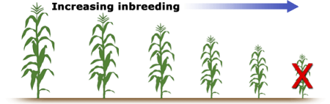
Through increasing homozygosity, inbreeding brings together identical alleles at a locus. Homozygosity permits the expression of recessive alleles that may have been previously masked by heterozygosity in the parent generation. If recessive alleles are less favorable than dominant ones, the overall fitness of the individual decreases. Inbreeding is often detrimental because it increases the appearance of lethal and deleterious recessive traits. The term inbreeding depression describes the decrease in fitness or performance that often accompanies inbreeding or random genetic drift. Recall that fitness is the relative ability of an individual to survive and reproduce to contribute its genes to the next generation. Inbreeding depression is further described in the next section.
Plant stature, vigor, yield and other traits decline with increasing inbreeding, although significant differences exist among species for the amount of inbreeding depression expressed—ranging from minimal among self-pollinated crops such as oat and wheat to severe in cross-pollinated polyploid species such as alfalfa, whereby homozygous genotypes do not survive (Fig. 4). Table 4 on the next screen summarizes some general differences between outbreeders and inbreeders.
Outbreeders vs. Inbreeders
| Outbreeder | Inbreeder |
|---|---|
| Has crossing mechanism, approaches random mating | Closed flowering, approaches regular selfing |
| Individuals heterozygous at many loci | Individuals approach homozygosity |
| Variability distributed over the population | Variability mostly between component lines |
| Carries deleterious recessives | Deleterious recessives tend to be eliminated |
| Intolerant of inbreeding | Tolerant of inbreeding |
| Much heterozygote advantage (epistasis, overdominance) | Less heterozygote advantage |
Inbreeding Depression
Inbreeding Depression and Homozygosity
Inbreeding results in increased homozygosity. In cross-pollinated species, increased homozygosity results in inbreeding depression or reduced performance. Symptoms of inbreeding depression may include:
- Reduced plant vigor
- Smaller plant size
- Decline in fertility
- Suppressed seed production
- Decreased pollen production
- Inferior seed quality
- Greater susceptibility to insect or pathogen damage or
- Poorer standability.
Why? With increased homozygosity, expression of deleterious recessive alleles may be revealed by fixation that had been masked by more favorable dominant alleles, or it can be caused by overdominance in which homozygotes are less fit, resulting in poorer performance.
The severity of inbreeding depression varies with the species and genotype. If the inbreeding depression is too severe, it may be difficult or impractical to maintain or propagate inbred lines by seed. In such cases, some heterogeneity must be maintained or other propagation means used.
Over-dominance: The phenotype of the heterozygous progeny is greater than either parent.
Mating Systems
The frequency of homozygotes in a population can be increased using any of several mating systems:
- Self-pollination—Repeated self-pollination is routinely used to develop pure lines of self-pollinating crops. It can also be applied to cross-pollinating species to obtain inbred lines. Like pure-lines in self-pollinated species, inbred lines are homozygous at nearly all loci.
- Half-sib mating—Plants having one parent in common are mated. The pollen source is random from the breeding population, but the female plants are identifiable.
- Full-sib mating—Plants having both parents in common are crossed.
- Backcrossing—A method in which a hybrid is mated to one of its parents, the recurrent parent, resulting in a backcross 1 (BC1) population. The resulting backcross offspring are repeatedly crossed to the recurrent parent.
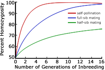
The inbreeding coefficient increases more rapidly with matings among more closely related individuals. The first three mating systems listed above are compared in Fig. 5. In each case the initial value of the inbreeding coefficient is assumed to be F0 = 0. Backcrossing—like self-fertilization—can be one of the most extreme forms of inbreeding.
Interpret the trends shown on the graph in Fig. 5.
After the 6th generation, what is the percent homozygosity in the half-sib and in the full-sib mating systems?
List the circumstance(s) under which the breeder would develop inbred lines using the half-sib mating or the full-sib mating system rather than self-pollination.
The challenge for the plant breeder is to develop inbred lines that can be maintained and are sufficiently homozygous to generate reliably superior and uniform progeny when mated to produce the hybrid cultivar. Inbred lines can be developed from any heterogeneous population. Heterogeneity is essential to obtain variability for important traits. Without variability for the characters of interest, the breeder cannot make selections or breeding progress.
Degree of Relatedness of Individuals
The coefficient of relatedness (rIJ) is a measure of the degree of relatedness between individuals (Table 5). It is the proportion of genes shared between two individuals I and J due to common descent (e.g., identical by descent). It ranges from -1.0 (no genes in common, at least among the genetic markers assessed) to +1.0 (vegetative clones). For example, the value of rIJ for a parent and each of their progeny is 0.5 for a sexually reproducing species because half of each offspring’s genes come from each parent. In the case of full-siblings the value of rIJ is also 0.5, but on average because siblings receive half of their genes from each of the same pair of parents, but the haploid set of genes in each parental gamete is a random sample of half of the parental genome due to recombination (Conner and Hartl 2004).
| Mating Systems | rIJ |
|---|---|
| Self-pollination*, vegetative clones, doubled haploids | 1.0 |
| Parents and offspring | 0.5 |
| Full siblings | 0.5 |
| Half siblings | 0.25 |
*After selfing for many generations
Heterosis
Heterosis or Hybrid Vigor
When inbred lines of cross-pollinating species are mated, their progeny are often superior to either or both of the parents for one or more characters, a phenomenon referred to as hybrid vigor or heterosis. Recall that genetic drift is random, so that different inbred lines or subpopulations tend to be fixed for different alleles at various loci; when they are intermated, the F1 population will be highly heterozygous. Heterosis is the opposite of inbreeding depression—heterosis is commonly expressed as
- Improved plant vigor,
- Greater plant size, and/or
- Increased productivity.
The performance of a hybrid relative to its parents can be described in two ways: mid-parent heterosis is the performance of a hybrid compared with the average of the performance of its parents; high-parent heterosis is a comparison of the performance of the hybrid with that of the best parent:
[latex]\text{mid-point heterosis (%)} = \frac{F_{1} - MP}{MP} \times 100[/latex]
Where:
- F1 = performance of the hybrid
- MP = average performance of the parents (Parent 1 + Parent 2)/2
- HP = performance of the best parent
Dominance vs. Overdominance Hypothesis
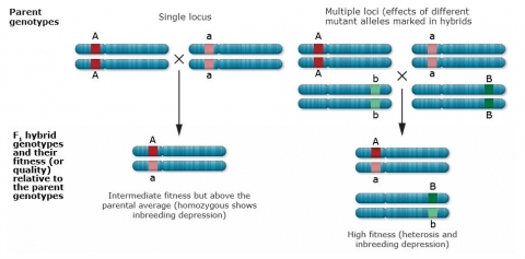
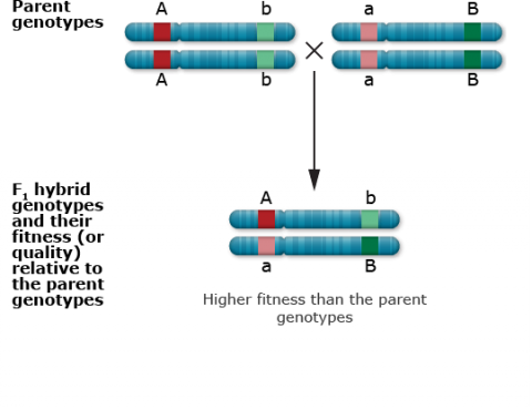
Heterosis tends to be greatest in the progeny of diverse genotypes. There are two common explanations for this phenomenon:
- Dominance hypothesis—Heterosis results from the complete or partial dominance of favorable alleles at various loci.
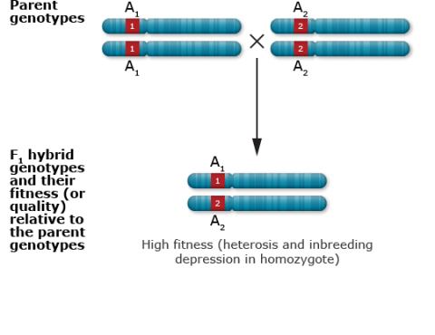
- Overdominance hypothesis—Heterosis reflects the superior performance of the heterozygote over either homozygote.
The next few pages provide a summary of the dominance and overdominance hypotheses from Charlesworth and Willis (2009). Note the differences between models for a single locus and those describing multiple loci. They include a third model that involves deleterious alleles at closely linked loci and focuses on so-called “pseudo-overdominance”, which will not be further discussed here.
Complete dominance
The phenotype of the heterozygous progeny equals the phenotype of the homozygous dominant parent.

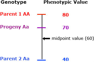
Partial (incomplete) dominance
The heterozygous progeny has a phenotypic value greater than that of the midparent value, but less than that of the homozygous dominant parent.
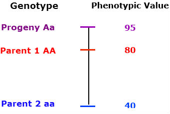
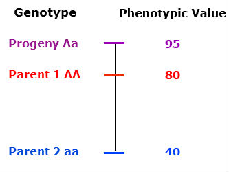
Overdominance
The phenotype of the heterozygous progeny is greater than either parent.
Main Genetic Hypothesis
Recessive deleterious mutations
Recessive deleterious mutations at closely linked loci
Single locus with heterozygous advantage
Heterozygote Advantage
Heterozygote advantage is a term that is frequently confused with heterosis. However, heterozygote advantage is a synonym of overdominance, and refers to a condition in which the heterozygous genotype has a higher phenotypic value (especially for fitness) than for either homozygous genotype. Heterosis is usually due to a number of loci that control quantitatively inherited traits, although depending on the situation it could be due to phenotypes controlled by either single genes or polygenic traits. In contrast, heterozygote advantage describes effects at a single locus (Conner and Hartl 2004). Compare the circumstances for these two concepts in Table 6.
| Subpopulations | ||
|---|---|---|
| Small and isolated | Crossed with each other | |
| Genotypic frequencies | Highly homozygous | Highly heterozygous |
| Fitness | Low | High |
| Fitness effects | Inbreeding depression | Heterosis or hybrid vigor |
| Cause for fitness effects | Deleterious recessives expressed or loss of heterozygote advantage | Deleterious recessives masked or occurrence of heterozygote advantage |
Genetics of Heterosis and Inbreeding Depression
Whatever genetic mechanisms can explain heterosis must also be able to explain inbreeding depression. Let’s take a look at hypothetical numeric examples of these two hypotheses to show how each can explain both.
In the following examples we will use a scenario where six genes control a certain quantitative characteristic.
Favorable Dominant Alleles Theory (with complete dominance at each locus)
- Heterosis The homozygous recessive genotype, aa bb cc dd ee ff has a value of 40. One dominant allele at any of the six genes increases the value by 10, that is, N_=+10.The following two homozygous parents are crossed. Each has a value of 70 because of having three loci with dominant alleles [40+(3)(10)=70].
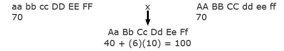 Note that the F1 has a value of 100 because of having six loci with dominant alleles (40 + (6)(10) = 100).
- Inbreeding depressionInbreeding depression can be explained with the accumulation of favorable dominant alleles mechanism. If we self the Aa Bb Cc Dd Ee Ff individuals that have a value of 100, we will get a population of individuals as follows:
Table 7 Percentage of individuals Number of loci with at least one dominant allele 17.80% 6 35.60% 5 29.66% 4 13.18% 3 3.30% 2 0.44% 1 0.02% 0
This gives an overall population mean value of 85. This is lower than the value of the Aa Bb Cc Dd Ee Ff parental individuals, thus showing depression upon inbreeding.
Although conclusive evidence to support either of these hypotheses remains elusive, the dominance hypothesis has been more widely accepted. However, it is recognized that a gene’s effect is determined by its effect in combination with:
- Other alleles at the same locus,
- Itself (when homozygous),
- Genes at other loci (epistasis), and
- Closely linked genes.
Thus, dominance, overdominance, and epistasis, most likely all contribute to heterosis.
Overdominance Theory
- Heterosis: The genotype aa bb cc dd ee ff has a value of 40.The homozygous dominant allele at any locus increases the value by 7 over the homozygous recessive allele, i.e., NN = +7. Heterozygous at any locus increases the value by 10 over the homozygous recessive, i.e. Nn = +10. The following homozygous parents are crossed; each has a value of 61 because of having three loci with homozygous alleles [40 + (3)(7) = 61]. The F1 has a value of 100 because of having six heterozygous loci.
- Inbreeding depression: Inbreeding depression can be explained with overdominance. If we self the Aa Bb Cc Dd Ee Ff individuals that have a value of 100, we will get a population of individuals with a mean value of 85 (see table above). As was the case for the “favorable dominant alleles theory”, this value is lower than the value of the Aa Bb Cc Dd Ee Ff parental individuals, thus showing depression upon inbreeding.
Genetic Analysis
Molecular techniques are now being used to try to shed more light on the mechanisms involved in heterosis. In a study published in 2006, Swanson-Wagner et al. assayed the gene expression of 13,999 maize genes from seedling plants of two inbred parents and their F1 hybrid. When comparing the three genotypes they found 1,367 of the genes produced significantly different amounts of messenger ribonucleic acid (mRNA), which performs an essential role in protein synthesis.
Analysis of these genes showed that 78 percent of them had additive gene action, 15 percent showed either high-parent or low-parent dominance, and 3 percent showed either overdominance or underdominance. (The other 45 genes showed non-additive gene action but with the statistical analysis used these genes could not be classified as dominant, overdominant, or underdominant.) The experiment analyzed individual genes and was not designed to evaluate interactions among the genes, so epistasis could not be measured.
This study involved only two maize inbred lines and their hybrid offspring and the evaluation was based on tissue from seedling plants. Different genes will be active during different parts of the life cycle of the maize plant and further studies will most likely show differential gene action among different genes. Likewise, different parents and hybrids and different species may well show very different gene action patterns among the same genes that were tested in this study. With just this one experiment, where nearly 14,000 genes were evaluated, we can see that heterosis is complex and that multiple types of gene action are involved. Molecular methods in the context of hybrid breeding will be discussed in detail in the molecular plant breeding course.
When two genetically different parents are mated, heterosis is observed in their F1 progeny.
- All seed and forage species express some level of heterosis.
- Most cross-pollinated species express greater heterosis than do self-pollinated species.
Because of the expense in producing hybrid cultivars, hybrid cultivars are generally developed only in those crops in which the level of heterosis results in significantly better performance.
References
Charlesworth, D. and J.H. Willis. 2009. The genetics of inbreeding depression. Nature Reviews Genetics 10: 783-796.
Conner, J. K., and D.L. Hartl. 2004. A Primer of Ecological Genetics. Sinauer Associates, Sunderland, MA.
Falconer, D.S. and T.F.C. Mackay. 1996. Introduction to Quantitative Genetics. 4th edition. Longman Pub. Group, Essex, England.
Pierce, B.A. 2010. Genetics: A Conceptual Approach. 3rd edition. W.H. Freeman, New York, NY.
Simmonds, N.W. and J. Smartt. 1999. Evolution of Crop Plants. 2nd edition. Longman, Essex, UK.
Swanson-Wager, R.A., Y. Jia, R. DeCook, L.A. Borsuk, D. Nettleton, and P.S. Schnable. 2006. All possible modes of gene action are observed in a global comparison of gene expression in a maize F1 hybrid and its inbred parents. PNAS 103:6805-6810.
Evaluation of the homogeneity of variance by calculating a Chi-squares value with the formula given in the "Mean Comparisons" module.
A statistical artefact that is due to the deviation of estimates from true values by random error. In a mapping experiment, the loci that are deemed significant are enriched for those in which the estimated effects benefit from random error that happens to fall in the right direction. Therefore, significant QTLs are disproportionately those in which the effect sizes are inflated by chance.
The binomial and Poisson distributions are related. The binomial distribution calculates the probability of a certain number of events occurring of two possible options. For instance, the number of times you will have three heads in a total of ten coin tosses.
Evaluation of the homogeneity of variance by calculating a Chi-squares value with the formula given in the "Mean Comparisons" module.
Abundance of a specific allele at a locus in a population
(1) Plants comprising the population are genetically identical.
(2) Population is comprised of genetically identical plants.
Condition that exists in a population of individuals with the same genotype.
A term that refers to the metabolism of a living organism and the array of biochemical pathways and processes
A transformation useful on data collected of proportions or percentages. These data may be transformed by taking the inverse of the sine or arcsine of the number.
A localized group of actively dividing cells from which permanent specialized tissues differentiate.
