
Chapter 6: Population Genetics
Laura Merrick; Kendra Meade; Arden Campbell; Deborah Muenchrath; and William Beavis
Introduction
Population genetics is a sub-discipline of genetics that characterizes the structure of breeding populations. The forces of mutation, migration, selection and genetic drift will alter the structure of populations. In this introductory module we will focus on characterizing population structure at a single locus. In more advanced modules you will learn how to characterize populations based on the multi-dimensional space determined by multiple loci throughout the genome.
- Understand the importance of a reference population.
- Become familiar with modeling and estimation of genetic variation.
- Understand the principles of allele frequency, genotype frequency, and genetic equilibrium in populations.
- Be aware of the conditions required for Hardy-Weinberg Equilibrium (HWE).
- Examine the forces that cause deviations from HWE.
Two possible challenges are described in the following scenarios:
Scenario 1—Fate of a Transgene
Imagine a community of small farms in a valley located in the highlands of Central America. The farmers of this community produce grain from an open-pollinated maize variety that is adapted to their preferred cultural practices. They also select partial ears from about 5% of their better performing plants to be used for seed in their next growing season.
One day, a truck filled with seed of a transgenic insect-resistant hybrid overturns on the highway while passing through the valley. 99.999% of the seed is recovered, but about 500 kernels remain in a farmer’s 10-acre field adjacent to the highway. The transgenic seeds germinate and grow to maturity alongside the planted open-pollinated variety. You are asked to determine the fate of an insect-resistant transgene in this valley.
Scenario 2—Fixation of an Allele
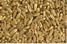
Imagine a naturally occurring allele at a locus that regulates the structure of carbohydrates in the wheat kernel; with the allele the carbohydrates in the kernel have low glycemic indices. For the last 100 years hard-red winter wheat varieties have not been selected for low glycemic indices, but with the emergence of a Type II diabetes epidemic, there is a demand for low glycemic carbohydrates in hard-red winter wheat varieties. How will you develop a breeding population in which this allele is fixed, that is the frequency of this allele = 1.0?
Fields of Genetics

These challenges are fundamentally about population genetics. In this section, you have the opportunity to successfully address these types of challenges by learning how to model and estimate allelic frequencies and the forces that affect population structures. In the study of population genetics, the focus shifts away from the individual (which is the focus for transmission genetics) and the cell (which is the focus for molecular genetics) to emphasis on a large group of individuals—a Mendelian population—that is defined as a group of interbreeding individuals who share a common set of genes.
This module will include a discussion of inbreeding, which is one type of mating of individuals that is often of particular significance to plant breeders.
Inbreeding is the mating of individuals that are more closely related than individuals mated at random in a population. Self-pollination (mating of an individual to itself) represents the most extreme form of inbreeding.
Reference Population
Goals
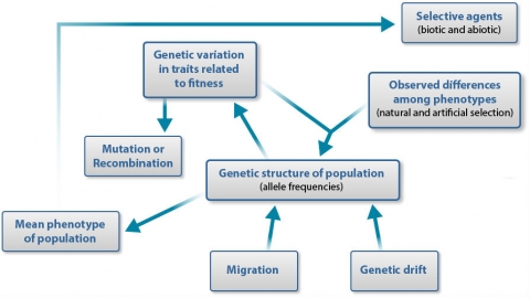
Population genetics has three major goals, all of which are interrelated (Conner and Hartl, 2004):
- Explain the origin and maintenance of genetic variation.
- Describe the genetic structure of populations, i.e., the patterns and organization of genetic variation.
- Recognize the mechanisms that cause changes in allele and genotypic frequencies.
Similar to quantitative genetics, population genetics is concerned with application of Mendelian principles and is amenable to mathematical treatment. Understanding population genetics will require you to apply concepts from high school algebra.
Description
In order to understand the genetic structure of a population, it is necessary to establish a standard reference population so that the breeding population can be characterized relative to the standard.
Consider an ‘ideal’ population that is infinitely large. Further consider development of sub-populations as in Figure 6, described in Falconer and Mackay (1996).
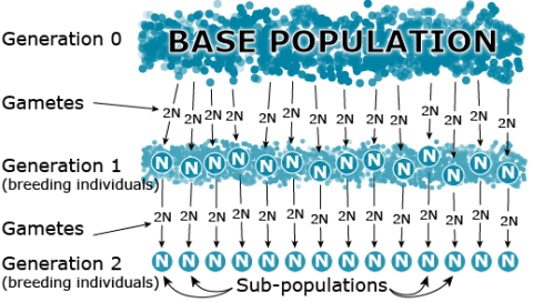
Note that the sub-populations depicted in the figure above are based on a genetic sampling process that is affected by reproductive biology of the species. The reproductive mode of most plant species can be classified as sexual or asexual Species that reproduce sexually are generally categorized into three types of mating systems — primarily cross-pollinated, primarily self-pollinated, or a mixture of self- and cross-pollinated. Asexual modes of reproduction include three main categories: vegetative or clonal propagation, and apomixis. Under different mating systems (e.g., random vs. inbreeding) different genotypic frequencies will be generated from the same allele frequencies. With sexually reproducing individuals, mating combines alleles in the pool of haploid gametes produced by meiosis into genotypes in the diploid individuals.
In the ideal model population depicted in Fig. 8, we make the following assumptions:
- The base population is extremely large (too large to count)
- No migration between sub-populations
- Non-overlapping generations
- Number of breeding individuals is the same in each sub-population
- Random mating within a sub-population
- No selection
- No mutation
Models such as that shown above are theoretical abstractions. Models provide methods to simulate real-life situations and they are used for two principal reasons: 1) to reduce complexity, allowing underlying patterns to become more visible and 2) to make specific predictions to test with experiments or observations (Connor and Hartl 2004).
Discussion
Discuss the two challenges described earlier with respect to each reference population:
For Scenario 1—Fate of a Transgene, characterize the breeding population. Assume that there are 100 10-acre farms in the Central American valley, where farmers plant about 10,000 maize kernels per acre.
For Scenario 2—Fixation of an Allele, determine how many hard red winter wheat varieties exist for the Southern Great Plains region. The number can include all historical varieties grown in the region. Assume that you have identified one additional ancient accession of hard red winter wheat that has the desirable allele for low glycemic carbohydrates. Assume that these varieties represent the lines you will use for your basic breeding population. Characterize this breeding population.
Allele and Genotypic Frequencies
Model
We first model a single locus with only two alleles (e.g., presence or absence of a transgene) in an ideal breeding population of diploid individuals. Define the following:
- N = Number of breeding individuals in a sub-population (population size)
- t = Time in generations with base population at t0
- q = Frequency of a particular allele at a locus within a sub-population
- p = 1 – q = Frequency of other allele at a locus within a sub-population
- [latex]\bar{p}[/latex] = Frequency in the whole population (the mean of p)
- p0 = Frequency of p in the base population
- q0 = Frequency of q in the base population
Because of the assumptions associated with an ideal reference population,  = q0 at any stage or generation of the sampling process, so q0 can be used interchangeably with
  .
.
Equations
The alleles, allele frequencies, genotypes and genotypic frequencies can be represented as follows:
| Alleles | Genotypes | ||||
|---|---|---|---|---|---|
| A | a | AA | Aa | aa | |
| Frequency | p | q | PAA | PAa | Paa |
Where,
[latex]p + q = 1[/latex]
and
[latex]P_{AA} + P_{Aa} + P_{aa} = 1[/latex]
The relationship between allele frequencies and genotype frequencies can be expressed as follows:
[latex]p = P_{AA} + \frac{1}{2}P_{Aa}[/latex]
and
[latex]q = P_{aa} + \frac{1}{2} P_{Aa}[/latex]
Hardy-Weinberg Equilibrium
Concept of Genetic Equilibrium
Plant breeders recombine and select the alleles present in the gene pool. The gene pool of a population is the total of all alleles within a population, and consists of all of the genes shared by individuals in the population. Gene pools are described in terms of allele and genotype frequencies. Knowing the frequency with which desired (or undesirable) alleles occur in the gene pool of the population influences the choice of breeding population(s), breeding method, and likelihood of progress. The breeding population must contain not only sufficient genetic variability to allow selection, but also have favorable alleles present in high enough frequencies to facilitate their selection and allow efficient breeding progress to occur.
- Allele frequency (often also called gene frequency) — the proportion of contrasting alleles present in the gene pool of a population.
- Genotype frequency — the proportion of various genotypes present in a population.
Assumptions
The frequencies of specific alleles and genotypes in a large, random mating population will reach equilibrium and will remain in equilibrium with continued random mating. This tendency toward equilibrium is the foundation of a model called the Hardy-Weinberg Law or Hardy-Weinberg Equilibrium (HWE). This law states that
The probability of two alleles uniting in a zygote is the product of the frequency of the alleles in the population
The law makes several assumptions.
- There are two alleles at a gene locus.
- The population is large (that is, the number of breeding individuals is in the hundreds, rather than in the tens).
- The population is random-mating.
Frequencies
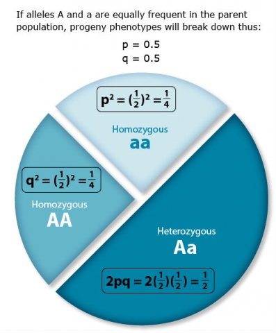
Hardy-Weinberg Equilibrium mathematically describes the relationship between allele frequency and genotype frequency. According to the Hardy-Weinberg law, if the frequencies of two contrasting alleles at a locus in the parent population are p and q, respectively, then [latex]p + q = 1[/latex], always; and genotype frequency in the progeny is [latex]p^2 + 2qp + q^2 = 1[/latex] or [latex]p^2 + 2qp + q^2 = 1[/latex].
For each of the following populations, indicate whether the Hardy-Weinberg Law would apply.
| Population | Does the Hardy-Weinberg Law apply? |
|---|---|
| Naturally self-pollinating species | YES NO |
| Naturally cross-pollinating species | YES NO |
| Limited population size | YES NO |
Locus Alpha has two contrasting gene forms or alleles (A and a) in a large, random-mating population. The population is at equilibrium.
space
The correct frequency of aa genotype following selection and random mating is 0.17. Selection for the A_ phenotype (or against the aa phenotype), shifts the allele and genotype frequencies. Here’s how the answer is determined:
- Initial population is 0.09 AA + 0.42 Aa + 0.49 aa
- Selection removes aa genotypes, so the unselected portion of the population is 0.09 AA + 0.42 Aa and the remaining individuals are all A_.
- Thus, setting p equal to the frequency of the A allele, and q equal to frequency of the a allele, the resulting allelic frequencies are now
[latex]\textrm{p} = \frac{\textrm{frequency of A in the AA genotype + frequency of A in the Aa genotype}}{\textrm{total allele frequencies of A and a}}[/latex]
[latex]p = \frac{0.09 \times 2 + 0.42 \times 1}{0.09 \times 2 + 0.42 \times 2}[/latex]
[latex]q=1-p=0.41[/latex] [latex]q=1-p=0.41[/latex]
- So, the frequency of the A allele is 0.59 and the frequency of the a allele is 0.41.
- Now, we can calculate the frequency of the aa genotype in the population after one generation of selection and subsequent random mating.
p2(AA) + 2pq(Aa) + q2(aa) = 1
(0.59)2 + 2 · 0.59 · 0.41 + (0.41)2 = 1
0.35 AA + 0.48 Aa + 0.17 aa = 1
Thus, the correct frequency of the aa genotype is 0.17.
Factors Affecting Equilibrium
Several factors may disturb the genetic equilibrium of a population.
- Mutation of an allele at the locus of interest.
- Natural or human selection may favor one allele over the other.
- Migration of alleles into or out of the population (for example, via an introduction of a different allele from another population, or loss of an allele through selection).
Generally, a population not in genetic equilibrium, but retaining two contrasting alleles at a single, independently-segregating (non-linked) locus, will be restored to equilibrium at that locus after just one generation of random mating.
Random-Mating Interference
What is the significance of the Hardy-Weinberg Law to plant breeders? The random-mating assumption is often violated in breeding populations because breeding populations are smaller than natural plant populations. Thus, a mating design that minimizes gamete (allele) sampling errors is an important consideration. The breeder must be aware of several factors:
- Self-pollinated population — allele frequency will remain in equilibrium (assuming a sufficiently large population, no selection, or other factors that disturb equilibrium). However, with each successive generation of self-pollination, the genotype frequency of homozygous loci will increase and the frequency of heterozygous loci will decrease. Ultimately, the heterozygous genotype will be eliminated from the population with continued selfing.
- Cross-pollinated population — sampling errors occur if plants in the population differ in their vigor, time of flowering, or mate more frequently with plants in close proximity.
- Selection for or against a particular allele will alter the allele and genotype frequencies of the population. Selection against a dominant allele (i.e., selection for homozygous recessive) will remove the dominant allele from the population in a single generation. Selection against a recessive allele will require more than a few generations to remove the recessive allele from the population because the homozygous dominant and heterozygous genotypes have indistinguishable phenotypes.
Scenarios
In addition to being able to estimate allele and genotype frequencies, the breeder also needs to understand the gene action affecting the character of interest.
The breeding of cross-pollinated crops differs from self-pollinated species because of differences in the structures of their gene pools and opportunity for genetic recombination.
| Reproductive mode | Individuals | Population |
|---|---|---|
| Self-pollinated | Homozygous | Homogeneous or heterogeneous |
| Cross-pollinated | Heterozygous | Heterogeneous |
For a given locus, an individual with a genotype of either AA or aa is homozygous for that gene and is known as a homozygote; the status of the gene is referred to as homozygosity. An individual with the genotype Aa is heterozygous for that gene and is called a heterozygote; the status is known as heterozygosity. In the case of polyploid individuals, those with the genotypes AAAA (tetraploid) or aaa (triploid) would be examples of homozygotes and those with genotypes of AAaa (tetraploid) or AAaaaa (hexaploid) would be examples of heterozygotes.
The terms homozygous and heterozygous are used to describe the status of single genes or all gene loci within an individual, not within a population. There may be many different alleles of a gene present in a population of individuals, but for each diploid individual, there are only two alleles per gene. For each individual, there is one allele from each parent and each allele per gene is present at corresponding loci on homologous chromosomes.
With regard to populations, a homogeneous population would be one in which all individuals in the population would have the same genotype and possess the same alleles for one or more genes. In contrast, a heterogeneous population would be characterized by differing alleles at one or more loci.
Note that a cross between two homozygous parents produces progeny that are homogeneous because all of the individual offspring are genetically identical. However, the offspring would be heterozygous for all loci for which different alleles occurred in the two parents.
Maize, the crop found in the first challenge, Scenario 1—Fate of a Transgene, is monoecious and is cross-pollinated.
Wheat, the crop found in the second challenge, Scenario 2—Fixation of an Allele, has bisexual flowers and is normally a self-pollinated crop.
| Flower Type | Self-Compatability or Dioecy/Monoecy | Crop Examples |
|---|---|---|
| Normally Cross-Pollinated | ||
| Bisexual Flowers | Self-Compatible | Sugarcane, Olive, Amaranth, Avocado, Onion, Carrot, Agave, Sunflower, Kiwi, Pearl millet, Reed canarygrass, Sweet potato |
| Bisexual Flowers | Self-Incompatible | Radish, Kale, Cabbage, Black mustard, Pineapple, Red Clover, White Clover, Apple, Pear, Cacao, Rye, Alfalfa, Birdsfoot trefoil, Sweet Potato, Buckwheat |
| Unisexual Flowers | Dioecious | Papaya, Fig, Hops, Hemp, Grape |
| Unisexual Flowers | Monecious | Mango, Cucumber, Squash, Watermelon, Yam, Rubber, Cassava, Castor bean, Maize, Banana, Coconut, Oil palm |
| Normally Self-Pollinated | ||
| Bisexual Flowers | Self-Compatible | Barley, Oats, Rice, Triticale, Wheat, Lettuce, Cowpea, Dry bean, Lentil, Chickpea, Peanut, Pea, Soybean, Sesame, Tomato, Tobacco, Coffee, Eggplant, Safflower, Flax, Peach |
| Predominantly Self-Pollinated, but also Cross-Pollinated to fairly high extent | ||
| Bisexual Flowers | Self-Compatible | Cotton, Sorghum, Rapeseed, Brown mustard |
Let’s examine the genetic structure of populations of self- and cross-pollinated species.
Scenario 1—Fate of a Transgene
Imagine a community of small farms in a valley located in the highlands of Central America. The farmers of this community produce grain from an open-pollinated maize variety that is adapted to their preferred cultural practices. They also select partial ears from about 5% of their better performing plants to be used for seed in their next growing season. One day a truck filled with seed of a transgenic hybrid overturns on the highway while passing through the valley. 99.999% of the seed is recovered, but about 500 kernels remain in a farmer’s 10-acre field adjacent to the highway. The transgenic seeds germinate and grow to maturity alongside the planted open-pollinated variety. You are asked to determine the fate of an insect-resistant transgene in this valley.
Scenario 2—Fixation of an Allele
Imagine a naturally occurring allele at a locus that regulates the structure of carbohydrates in the wheat kernel; with the allele, the carbohydrates in the kernel have low glycemic indices. For the last 100 years, hard-red winter wheat varieties have not been selected for low glycemic indices, but with the emergence of a Type II diabetes epidemic, there is a demand for low glycemic carbohydrates in hard-red winter wheat varieties. How will you develop a breeding population in which this allele is fixed, that is the frequency of this allele = 1.0?
Genetics of Cross-Pollinated Species
Because cross-pollinated species have evolved to outcross, individuals tend to be heterozygous at many loci and they usually perform best when that heterozygosity is maintained. This is a characteristic referred to as heterosis or hybrid vigor. When repeated self-pollination occurs in cross-pollinated species, homozygosity increases and plant vigor is reduced, a phenomenon called inbreeding depression. Heterosis and inbreeding depression will be further discussed in Lesson 6.
Several morphological and physiological features of cross-pollinated species promote cross-pollination. Let’s briefly review these.
- Monoecy — pistillate and staminate flowers occur on different sections of the same plant.
- Dioecy — pistillate and staminate flowers occur on different plants.
- Protandryorprotogyny — pistillate and staminate flowers mature at different times.
- Self-incompatibility — pollen from the same plant cannot effect fertilization or seed set.
- Male or female sterility — pollen or ovule does not function normally.
Genetics of Self-Pollinated Species
Self-pollinated species rarely hybridize naturally. Although cross-pollinating may occasionally occur, ovules of a self-pollinated plant are normally fertilized by pollen produced on that same plant. The result of repeated generations of selfing is that homozygosity is increased or maintained.
- Homozygous loci will remain homozygous.
- Heterozygous loci will segregate such that the frequency of homozygotes will increase at the expense of the frequency of heterozygotes with each generation of selfing.
With continued self-pollination, the heterozygotes will segregate, decreasing the proportion of heterozygotes in the population by half each generation. Notice that the homozygotes can only produce homozygotes.
| Generation | Heterozygosity (%) |
|---|---|
| F1 | 100.0 |
| F2 | 50.0 |
| F3 | 25.0 |
| F4 | 12.5 |
| F5 | 6.25 |
| F6 | 3.12 |
For each successive generation of offspring resulting from one F1 individual, by the F8 generation, the population is essentially homozygous. When no further segregation for the trait occurs, all progeny derived from that F1 will “breed true” because they are homozygous for the trait. The proportion of plants that are expected to be heterozygous at any gene when starting with a heterozygous F1 and selfing can be determined by using the formula (½)n, where n = the number of segregating generations, e.g., in F2 n = 1 and in F5 n = 4.
Proportion of homozygous plants in any generation is then given by 1 − (½)n which when algebraically converted is equal to: [latex]\frac{2^n - 1} {2^n}[/latex]
How does a locus become heterozygous? A contrasting allele can be acquired when a plant out-crosses or when a mutation occurs. Each successive self-pollination thereafter will reduce heterozygosity by half. Breeders rely on the natural tendency of self-pollinated crops to become homozygous to obtain lines that exhibit uniformity in characters that affect appearance and performance.
Notice how rapidly populations lose heterozygosity with selfing. For self-pollinated crops, one of the breeder’s objectives is usually to develop pure lines. Since pure lines are homozygous, their rapid loss of heterozygosity speeds cultivar development. Some background heterozygosity may remain in a pure line, but the line is sufficiently homozygous to provide the uniformity in characters required for reliable and predictable appearance and performance.
Allelic Effects
The tendency of a species to self-pollinate or outcross influences allelic and genotypic frequencies in the population. In a self-pollinated homozygous population, the effect of a gene (allele) is determined by the gene’s effect in combination with itself and with alleles at other loci. What determines the effect of a gene in a cross-pollinated population?
Effect or fate of an allele in a cross-pollinated population is determined by its effect
- in combination with other alleles at the same locus
- additive effects
- dominance effects
- overdominance effects
- in combination with alleles at other independent loci (epistatic effects)
- in combination with alleles at closely linked loci
One difference between a self-pollinated and a cross-pollinated population is that in the cross-pollinated population there is constant inter-crossing. Thus, recombination and rearrangement of alleles and expression of dominance and epistatic effects occur.
Review gene action or gene interactions, such as epistasis in the next screens.
Gene Action
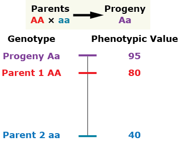
There are several general types of gene action. The type of gene action and the alleles present for a given gene affect the phenotype. Let’s consider the gene action as indicated by the phenotype of a diploid individual heterozygous at the given single locus compared to the phenotype of its parents.
Additive gene action (no dominance)
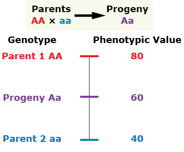
Complete Dominance
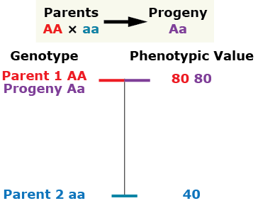
Partial (incomplete) dominance
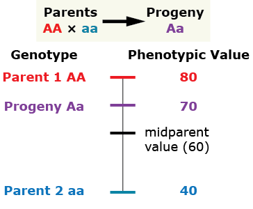
Over-Dominance
Gene Interactions
When multiple genes control a particular trait or set of traits, gene interactions can occur. Generally, such interactions are detected when genetic ratios deviate from common phenotypic or genotypic proportions.
- Pleiotropy — Genes that affect the expression of more than one character.
- Epistasis — Genes at different loci interact, affecting the same phenotypic trait.
Epistasis occurs whenever two or more loci interact to create new phenotypes. Epistasis also occurs whenever an allele at one locus either masks the effects of alleles at one or more other loci or if an allele at one locus modifies the effects of alleles at one or more other loci. There are numerous types of epistatic interactions.
Epistasis is expressed at the phenotypic level. It is important to note that genes that are involved in an epistatic interaction may still exhibit independent assortment at the genotypic level. In the case of two completely dominant, non-interacting (i.e., no linkage) genes, all of the deviations observed in results involving epistatic interactions are modifications of the expected 9:3:3:1 ratio.
Describe a natural cross-pollinated population as to its heterozygosity, heterogeneity, and effect of inbreeding. For each of the following, select the best terms to complete the statement.
Proof
The proof of Hardy-Weinberg Equilibrium (HWE) requires the following assumptions (Falconer and Mackay, 1996):
- Allele frequency in the parents is equal to the allele frequency in the gametes
- Assumes normal gene segregation
- Assumes equal fertility of parents
- Allele frequency in gametes is equal to the allele frequency in gametes forming zygotes
- Assumes equal fertilizing capacity of gametes
- Assumes large population
- Allele frequency in gametes forming zygotes is equal to allele frequencies in zygotes
- Genotype frequency in zygotes is equal to genotype frequency in progeny
- Assumes random mating
- Assumes equal gene frequencies in male and female parents
- Genotype frequencies in progeny do not alter gene (allele) frequencies in progeny.
- Assumes equal viability
For a two allele locus in a population in HWE: [latex]P_{AA}= p^2[/latex]; [latex]P_{Aa} = 2_{pq}[/latex]; [latex]P_{aa} = q^2[/latex]
Proof
HWE at a given genetic locus is achieved in one generation of random mating. Genotype frequencies in the progeny depend only on the gene (allele) frequencies in the parents and not on the genotype frequencies of the parents.
If a population is in HWE, relationships between frequencies of alleles and genotypes may be derived as depicted in figure 13.
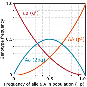
As shown in figure 13, in HWE:
- frequency of heterozygotes does not exceed 0.5
- heterozygotes are most frequent genotype when p or q are between 0.33 and 0.66
- very low allele frequency should result in very low frequency of homozygotes for that allele
- if there are only two alleles at a locus in the population, p+q=1.
A chi-square test is typically used to determine whether or not a population varies significantly from Hardy-Weinberg expectations. The Hardy-Weinberg formula is useful in describing situations where mating is completely randomized. But more commonly, mating is not at random and populations are subjected to other forces, such as mutation, migration, genetic drift, and selection. Linkage can also have a significant effect on gene frequencies.
Forces Affecting Population Structures
Descriptions
Non-Random Mating
Two methods of non-random mating that are important in plant breeding are assortative mating and disassortative mating.
Assortative mating occurs when similar phenotypes mate more frequently than they would by chance. One example would be the tendency to mate early x early-maturing plants and late x late maturing plants. The effect of assortative mating is to increase the frequency of homozygotes and decrease the frequency of heterozygotes in a population relative to what would be expected in a randomly mating population. Assortative mating effectively divides the population into two or more groups where matings are more frequent within groups than between groups.
Disassortative mating occurs when unlike or dissimilar phenotypes mate more frequently than would be expected under random mating. Its consequences are in general opposite those of assortative mating in that disassortative mating leads to an excess of heterozygotes and a deficiency of homozygotes relative to random mating. Disassortative mating can also lead to the maintenance of rare alleles in a population. For example, in self-incompatible species, an individual will only mate with another individual that differs in the self-incompatibility loci. This is a type of disassortative mating, resulting in a great alleleic diversity in the self-incompatibility loci. It is an effective mechanism to maintain heterozygosity and prevent inbreeding.
Scenario 2—Fixation of an Allele
Forces Affecting Allele Frequency
Factor Categories
The factors affecting changes in allele frequency can be divided into two categories: systematic processes, which are predictable in both magnitude and direction, and dispersive processes, which are predictable in magnitude but not direction. The three systematic processes are migration, mutation, and selection. Dispersive processes are a result of sampling in small populations.
| Systematic Processes | Dispersive Processes |
| Migration | Small Population Size |
| Mutation | |
| Selection |
Migration
Clearly, the first challenge described in the introduction represents a case of migration. A new set of genes in a developed transgenic hybrid have been introduced into an open pollinated variety of maize. When discussing population genetics, migration is also sometimes referred to as gene flow, a concept that is often used interchangeably with migration by population geneticists. However, the term migration means the movement of individuals between populations, whereas gene flow is the movement of genes between populations. New genes would be established in the population if the immigrant successfully reproduces in its new environment, but if it doesn’t reproduce migration would still have occurred while gene flow would not.
Assume a population has a frequency of m new immigrants each generation, with 1− m being the frequency of natives. Let qm be the frequency of a gene in the immigrant population and q0 the frequency of that gene in the native population. Then the frequency in the mixed population will be:
[latex]q_1 = mq_m +(1-m)q_0[/latex]
[latex]q_1 = m(q_m - q_0) + q_0[/latex]
The change in gene frequency brought about by migration is the difference between the allele frequency before and after migration
[latex]\Delta q = q_1 - q_0[/latex]
[latex]\Delta q = m (q_m - q_0)[/latex]
Thus the change in gene frequency from migration is dependent on the rate of migration and the difference in allele frequency between the native and immigrant population. Migration or gene flow can introduce new alleles into a population at a rate and at more loci than expected from mutation. It can also alter allele frequencies if the populations involved have the same alleles but not in the same proportions. Thus the effect of migration on changes in allele frequency depends on differences in allele frequencies (migrants vs. residents) and the proportion of migrants in the population.
Scenario 1—Fate of a Transgene
Mutation
Mutations are the source of all genetic variation. Loci with only one allelic variant in a breeding population have no effect on phenotypic variability. While all allelic variants originated from a mutational event, we tend to group mutational events in two classes: rare mutations and recurrent mutations where the mutation occurs repeatedly.
Rare Mutations
By definition, a rare mutation only occurs very infrequently in a population. Therefore, the mutant allele is carried only in a heterozygous condition and since mutations are usually recessive, will not have an observable phenotype. Rare mutations will usually be lost, although theory indicates rare mutations can increase in frequency if they have a selective advantage.
Fate of a Single Mutation
Consider a population of only AA individuals. Suppose that one A allele in the population mutates to a. Then there would only be one Aa individual in a population of AA individuals. So the Aa individual must mate with a AA individual.
AA x Aa → 1AA:1Aa
From Li (1976; pp 388), this mating has the following outcomes:
- No offspring are produced in which case the mutation is lost.
- One offspring is produced: the probability of that offspring being AA is 1/2 so the probability of losing the mutation is 1/2.
- Two offspring are produced: the probability of them both being AA is 1/4 so the probability of losing the mutation is 1/4.
If k is the number of offspring from the above mating then the probability of losing the mutation among the first generation of progeny is (1/2)k.
The probability of losing the gene in the second generation can be calculated by making the following assumptions:
- Number of offspring per mating is distributed as a Poisson process (which means that they follow a stochastic distribution in which events occur continuously and independently of one another).
- With the average number of offspring per mating = 2.
- New mutations are selectively neutral.
With these assumptions, the probabilities of extinction are:
| Generation | Probability of Loss |
|---|---|
| 1 | 0.37 |
| 7 | 0.79 |
| 15 | 0.89 |
| 31 | 0.94 |
| 63 | 0.97 |
| 127 | 0.98 |
Recurrent Mutations
Let the mutation frequencies be:
Mutation rate: [latex]A\xrightarrow{u}a[/latex]
Frequency: [latex]p_0\overleftarrow{v}q_0[/latex]
Then the change in gene frequency in one generation is:
[latex]\Delta q_0 = up_0 - vq_0[/latex]
at equilibrium
[latex]p_0u = q_0v[/latex]
[latex]q_0 = \frac{u}{v + u}[/latex]
Conclusions:
- Mutations alone produce very slow changes in allele frequency
- Since reverse mutations are generally rare, the general absence of mutations in a population is due to selection
Selection
Selection is one of the primary forces that will alter allele frequencies in populations. Selection is essentially the differential reproduction of genotypes. In population genetics, this concept is referred to as fitness and is measured by the reproductive contribution of an individual (or genotype) to the next generation. Individuals that have more progeny are more fit than those who have less progeny because they contribute more of their genes to the population.
The change in allele frequency following selection is more complicated than for mutation and migration, because selection is based on phenotype. Thus, calculating the change in allele frequency from selection requires knowledge of genotypes and the degree of dominance with respect to fitness. Selection affects only the gene loci that affect the phenotype under selection—rather than all loci in the entire genome—but it also would affect any genes that are linked to the genes under selection.
Effects of Selection
Change in allele frequency
The strength of selection is expressed as a coefficient of selection, s, which is the proportionate reduction in gametic output of a genotype compared to a standard genotype, usually the most favored. Fitness (relative fitness) is the proportionate contribution of offspring to the next generation.
Partial selection against a completely recessive allele
To see how the change in allele frequency following selection is calculated consider the case of selection against a recessive allele:
| Genotypes | ||||||
|---|---|---|---|---|---|---|
| AA | Aa | aa | Total | |||
| Initial Frequencies | p2 | 2pq | q2 | 1 | ||
| Coefficient of Selection | 0 | 0 | s | |||
| Fitness | 1 | 1 | 1-s | |||
| Gametic Contribution | p2 | 2pq | q2(1-s) | 1 – sq2 | ||
Frequency Equations
The frequency of allele a after selection is:
[latex]q_1 = \frac{q-sq^2}{1-sq^2}[/latex]
[latex]q_1 = \frac{q-sq^2}{1-sq^2}[/latex]
The change in allele frequency is then:
[latex]\Delta q = q_1 - q[/latex]
[latex]\Delta q = \frac{q-sq^2}{1-sq^2} -q[/latex]
In general, you can show that the number of generations, t, required to reduce a recessive from a frequency of q0 to a frequency of qt, assuming complete elimination of the recessive (s = 1) is:
[latex]t = \frac{1}{q_t} - \frac{1}{q_0}[/latex]
Discussion
Review the two challenges at the beginning of the lesson and then answer these questions:
- Allele Frequency—For Scenario 1, calculate the frequency of the insect-resistant transgene in the Central American maize farmer’s 10-acre field assuming that it is a) hemizygous and b) homozygous in the spilled hybrid seed. Remember that hemizygous means that the individual has only one single homologous chromosome, and therefore is neither homozygous nor heterozygous; in contrast homozygous means that there are two homologues.
- Allele Frequency—For Scenario 2, calculate the frequency of the allele responsible for low glycemic carbohydrates in the wheat breeding population, assuming the allele is not present in any wheat variety except one.
- Mutation—For Scenario 2, assume the mutation that produced the low glycemic allele was selectively neutral in the hard red-winter wheat breeding population. Why was that allele lost from all varieties that were developed over the last 100 years?
- Selection—In Scenario 1 a transgene (and likely other genes) is introduced into an open-pollinated variety in one farmer’s field. Determine Δq for the transgenic allele assuming that the allele is homozygous in the hybrid seed, the insect-resistant allele is completely dominant and the selective advantage of the allele is a) two to one (2:1) when the insect is present and b) one to one (1:1) when it is absent.
Scenario 1: Fate of a Transgene
Imagine a community of small farms in a valley located in the highlands of Central America. The farmers of this community produce grain from an open-pollinated maize variety that is adapted to their preferred cultural practices. They also select partial ears from about 5% of their better performing plants to be used for seed in their next growing season. One day a truck filled with seed of a transgenic hybrid overturns on the highway while passing through the valley. 99.999% of the seed is recovered, but about 500 kernels remain in a farmer’s 10-acre field adjacent to the highway. The transgenic seeds germinate and grow to maturity alongside the planted open pollinated variety. You are asked to determine the fate of an insect-resistant transgene in this valley.
Scenario 2: Fixation of an Allele
Imagine a naturally occurring allele at a locus that regulates the structure of carbohydrates in the wheat kernel; with the allele the carbohydrates in the kernel have low glycemic indices. For the last 100 years hard-red winter wheat varieties have not been selected for low glycemic indices, but with the emergence of a Type II diabetes epidemic, there is a demand for low glycemic carbohydrates in hard-red winter wheat varieties. How will you develop a breeding population in which this allele is fixed, that is the frequency of this allele = 1.0?
Small Population Size
Unlike the three systematic forces that are predictable in both amount and direction, changes due to small population size are predictable only in amount and are random in direction.
The effects of small population size can be understood from two different perspectives. It can be considered a sampling process and it can be considered from the point of view of inbreeding. The inbreeding perspective is more interesting, but looking at it from a sampling perspective lets us understand how the process works.
A particular sub-population is a random sample of N individuals or 2N gametes (for a diploid) from the base population. Therefore, the expected gene frequency of a particular allele in the sub-populations is q0 and the variance of q is [latex]\sigma^2_q = \frac{p_0q_0}{2N}[/latex]
Since q0 is a constant, the variance of the change in allele frequency (q1 − q0) is also: [latex]\sigma^2_{\Delta q} = \frac{p_0q_0}{2N}[/latex]
Examples
Example 1: Let q = 0.5 and N = 50, then [latex]\sigma_{q}^{2}= \frac{(0.5)(0.5)}{100}=0.0025[/latex]
Example 2: Let q = 0.5 and N = 4, then [latex]\sigma_{q}^{2}= \frac{(0.5)(0.5)}{8}=0.03125[/latex]
Consequences of small population size
- Random genetic drift: random changes in allele frequency within a subpopulation
- Differentiation between subpopulations
- Uniformity within subpopulations
- Increased homozygosity
Random Genetic Drift
Small Population Size
Random genetic drift refers to allelic frequencies that change through time (generations) due to errors and other random factors (i.e., not selection or mutation). When sample sizes are small, all genotypes may not be produced and then mate at expected frequency. The effective population size (Ne) of a population is a term used to describe the number of parents that actually contribute gametes to the next generation; not all individuals may contribute equally, thus resulting in genetic drift. Small populations are susceptible to genetic bottlenecks, which are sudden decreases in breeding population due to deaths, migration, or other factors. Small populations can be subject to so-called founder effects, which occur when a breeding population is small when initially founded, then increases in size but the gene pool is largely determined by the genes present in the original founders.
Rate of Change
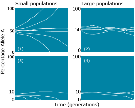
The rate of change due to random genetic drift depends on population size and allele frequency. As illustrated in the figure below, the more frequent the allele, the higher chances of being fixed and the smaller the population, the faster it will either move towards fixation or loss. In the absence of other forces:
- genetic drift leads to loss or fixation of alleles
- frequency of rare alleles would be expected to go to zero
- lower frequency of heterozygotes in later generations
- less genetic variation within subpopulations
- more genetic variation among subpopulations
Inbreeding and Small Populations
Inbreeding and Small Populations Inbreeding is the mating together of individuals that are related by ancestry. The degree of relationship among individuals in a population is determined by the size of the population. This can be seen by examining the number of ancestors that a single individual has:
Just 50 generations ago note that a single individual would have more ancestors than the number of people that have existed or could exist on earth.
Therefore, in small populations individuals are necessarily related to one another. Pairs mating at random in a small population are more closely related than pairs mating together in a large population. Small population size has the effect of forcing relatives to mate even under random mating, thus with small population sizes inbreeding is inevitable.
| Generation | Ancestors |
|---|---|
| 0 | 1 |
| 1 | 2 |
| 2 | 4 |
| 3 | 8 |
| 4 | 16 |
| 5 | 32 |
| 6 | 64 |
| 10 | 1,024 |
| 50 | 1,125,899,906,842,620 |
| 100 | 1,267,650,600,228,230,000,000,000,000,000 |
| t | 2t |
Identical Types
In finite populations there are two sorts of homozygotes: Those that arose as a consequence of the replication of a single ancestral gene — these genes are said to be identical by descent (Bernardo, 1996). If the two genes have the same function, but did not arise from replication of a single ancestral gene, they are said to be alike in state. It is the production of homozygotes that are identical by descent that gives rise to inbreeding in a small population.
Study Question 6
Scenario 2—Fixation of an Allele
Summary of Factors
Hardy and Weinberg discovered mathematically that genotype frequencies will reach an equilibrium in one generation of random mating in the absence of any other evolutionary force. If the conditions of equilibrium are met, the frequencies of different genotypes in the progeny will depend only upon the allele frequencies of the previous generation. If allele frequencies do not accurately predict genotype frequencies, then plants are mating in a non-random way or another evolutionary force is operating.
| Effect of level of variation | |||
| Within subpopulations | Among subpopulations | Affect all loci equally? | |
| Mutation | Increase | Increase | No |
| Migration (Gene flow) | Increase | Decrease | Yes |
| Random Genetic Drift | Decrease | Increase | Yes |
| Selection | Increase or decrease | Increase or decrease | Yes |
Within subpopulations the degree of genetic variation can be assessed by heterozygosity, while variation among subpopulations is measured by population differentiation. Mutation is the ultimate source of all genetic variation and it tends to increase variation both within and among subpopulations. But because most mutations are rare, the effect of mutation is slow relative to the change the other forces can effect. Migration or gene flow and random genetic drift are opposite in their effects: migration tends to increase variation within subpopulations but decrease it among subpopulations, and random drift does the opposite. In contrast, the effects of selection vary both within and between populations. For example, variation can decrease if one homozygote is favored, or may increase or be maintained if heterozygosity is advantageous. Selection acts on the phenotype so it will affect only those genes that control the trait under selection, as well as genes linked to those loci.
Schematic Overview
References
Bernardo, R., A. Murigneux, and Z. Karaman. 1996. Marker-based estimates of identity by descent and alikeness in state among maize inbreds. Theoretical and Applied Genetics 93: 262-267.
Conner, J. K., and D.L. Hartl. 2004. A Primer of Ecological Genetics. Sinauer Associates, Sunderland, MA.
Falconer, D.S. and T.F.C. Mackay. 1996. Introduction to Quantitative Genetics. 4th edition. Longman Pub. Group, Essex, England.
Hancock, J.F. 2004. Plant Evolution and the Origin of Crop Species. 2nd edition. CABI Publishing, Cambridge, MA.
National Institutes of Health. National Human Genome Research Institute. “Talking Glossary of Genetic Terms.” http://www.genome.gov/glossary/
Pierce, B. A. 2008. Genetics: A Conceptual Approach. 3rd edition. W.H. Freeman, New York.
Presence of different alleles, or contrasting gene forms, at corresponding loci on homologous chromosomes.
A method used to determine the response relationship of data. This method determines whether data is linear (form y=ax+b), parabolic (y=ax2+bx+c), or higher order.
The haploid, sexual generation or phase in the plant's life cycle that produces haploid gametes via mitosis.
Evaluation of the homogeneity of variance by calculating a Chi-squares value with the formula given in the "Mean Comparisons" module.
(1) A genotype that contains one dominant and one recessive gene or two different co-dominant genes (Aa,bB,CD).
(2) An individual that has two copies of the same allele at a locus, e.g., AA or aaa or AAAA.
Synonymous with in vitro propagation, especially in reference to enhanced axillary branching or adventitious plantlet regeneration. See also in vitro propagation.
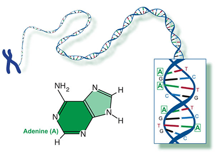
One of the building blocks of DNA or RNA, each of which contains a nitrogenous base attached to a five-carbon sugar that in turn is attached to one or more phosphate groups.
Introduction
Mutations
Mutations are the ultimate source of all genetic variation. Mutations can occur at all levels of genetic organization, classified mainly as either chromosome mutations or genome mutations. Chromosome mutations are discussed in this module. Chromosome alterations involve either single nucleotides or fragments of chromosomes and are either small-scale (one or a few nucleotides substituted, inserted, or deleted) or large-scale (deletions, insertions, inversions, or translocations involving large segments of chromosomes or duplications of entire genes). Genome mutations—involving changes in number of whole chromosomes or sets of chromosomes—will be covered separately in the module on Ploidy—Polyploidy, Aneuploidy, Haploidy.
Genetic variation—dissimilarity between individuals attributable to differences in genotype—that is generated by mutations is acted upon by various evolutionary forces. Evolutionary processes that alter species and populations include selection, gene flow (migration), and genetic drift—whether or not plants are cultivated or wild. Evolution can be defined as a change in gene frequency over time. The way that plants evolve is dependent on both genetic characteristics and the environment they face.
Genetic variation results from differences in DNA sequences and, within a population, occurs when there is more than one allele present at a given locus. Major processes that affect heritable variation in crop plants are topics emphasized throughout the lessons of this course. Changes in gene frequencies within populations caused by natural selection can lead to enhanced adaptation, while changes caused by human-directed selection can facilitate the development of useful genetic variability and selection of superior genotypes. Selection is the differential reproduction of the products of recombination—both within and between chromosomes.
Genetic Resources
Historically plant breeders seeking sources of variability were constrained in choice of parental materials or plant genetic resources that were interfertile within closely related gene pools. But a range of new techniques such as mutagenesis, genetic engineering (transgenic or transformed plants), and in vitro methods (tissue culture, doubled haploids, induced polyploids) expand the source and scope of variability that can be used in crop improvement.
Our expanding understanding of the molecular basis of genetics has provided insights and technologies that further not only our basic understanding of genes and their regulation, but also provide additional tools for crop improvement. Molecular techniques enable breeders to generate genetic variability, transfer genes between unrelated species, move synthetic genes into crops, and make selections at the molecular, cellular, or tissue levels. Combining these laboratory techniques with conventional field approaches can shorten the time required to develop new or improved cultivars. The importance and application of molecular technologies are rapidly increasing.
These topics mentioned above—mutations, gene expression, genetic markers, sources of genetic variation, genetic engineering, and molecular breeding methods—will be briefly mentioned in this module, but covered in greater detail in the later courses including Plant Breeding Methods, Molecular Genetics, and Biotechnology and Molecular Plant Breeding.
- Recognize how mutations are classified and inherited, as well as how mutations affect structure, processes, and products of genes and chromosomes.
- Understand the basic principles of transcription and translation.
- Become familiar with sources of genetic variation for cultivated plants, including crop gene pools and genetic engineering methods.
Mutations as Heritable Change
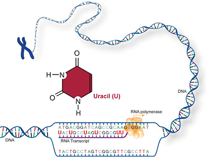
Without heritable variation, any trait favored by selection will not be passed on to offspring. Mutation is defined as heritable change in genetic information. Mutations entail modification of the nucleotide sequence of DNA and consist of any permanent alteration of a DNA molecule that can be passed on to offspring. DNA is a highly stable molecule and it replicates with a high degree of accuracy. However changes in DNA structure and replication errors can occur. Mutation involves modifications in the sequence of bases in DNA transmitted through mitosis and meiosis.
A nucleotide consists of a sugar molecule (ribose in RNA or deoxyribose in DNA) attached to phosphate group and a nitrogen-containing base. In DNA or RNA molecules, each strand has a backbone of sugar and phosphate groups (Fig. 17).
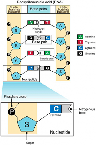
CHEMICAL BASES IN DNA AND RNA
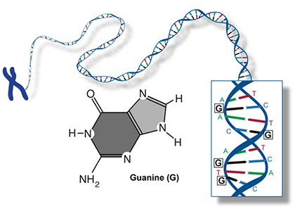
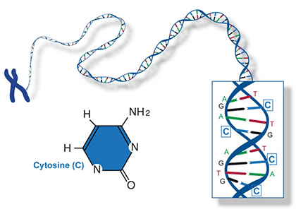
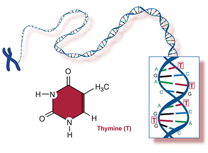
Two of the four nitrogenous bases in DNA—adenine (Fig. 13) and guanine (Fig. 14) are known as purines and the other two—cytosine (Fig. 15) and thymine (Fig. 16) are pyrimidines. Adenine, guanine, and cytosine are also found in RNA. Another pyrimidine known as uracil (Fig. 17) is the base used in RNA in place of thymine.
Some mutations occur in loci that encode for gene products such as proteins, and thus they may affect the processes of transcription, translation, or gene expression—processes that happen during the creation of proteins from the genetic code in DNA. But mutations also can occur in parts of the genome that do not code for any gene products (called noncoding DNA) or sequences that serve to control regulatory functions in the cell or chromosomes. For most loci, mutation changes allelic frequencies at a very slow rate and therefore consequences are negligible. Mutations may or may not change the phenotype of an organism. The majority of mutations that do occur are neutral in their effect and therefore do not have an influence on fitness. Some mutations are beneficial. But mutations can have deleterious effects, causing disorders or death.
Amino acids are a set of 20 different molecules used to build proteins. A peptide is one or more amino acids linked by chemical bonds (termed peptide bonds). Linked amino acids form chains of polypeptides (Fig. 18). The amino acid sequences of proteins are encoded in genes.
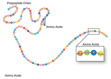
One or more polypeptides form the building blocks of proteins (Fig. 19). Proteins perform a variety of roles in cells.
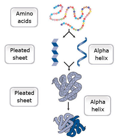
Primary protein structure is a sequence of a chain of amino acids.
Secondary protein structure occurs when the sequence of amino acids is linked by hydrogen bonds.
Tertiary protein structure occurs when certain attractions are present between alpha helices and pleated sheets.
Quaternary protein structure is a protein consisting of more than one amino acid chain
Types of Mutations
Classification of Mutations
Mutations can occur at all levels of genetic organization, ranging from simple base nucleotide pair alterations to shifts and rearrangements in sequences of nucleotides along fragments of chromosomes to changes in the number and structure of whole chromosomes.
A mutation is a change from one hereditary state to another, e.g., allele A mutates to allele a. For a given locus, the normal allele is referred to as the ‘wildtype’. Mutations are usually recessive and therefore their effects are hidden in heterozygotes. There are a number of common ways to classify mutations, including the following:
- causal agent
- rate or frequency of occurrence
- kind of tissue involved and its type of inheritance
- impact on fitness or function, or
- molecular structure and scale of the mutation.
Spontaneous vs. Induced Mutations
Depending on the cause, mutations can be either spontaneous or induced:
- Spontaneous mutations occur naturally with no intentional exposure to a mutagen. Spontaneous mutations can result from copying errors made during cell division.
- Induced mutations are caused by mutagens, either chemicals or radiation.
RARE VS. RECURRENT MUTATIONS
Recall from the module on Population Genetics, mutational events in a population can be classified into two categories based on frequency of occurrence:
Rare mutations (also called non-recurrent mutations) are defined as those that occur infrequently in populations. Rare mutations are usually recessive and occur in a heterozygous condition so that their effect on the phenotype is not apparent. Rare mutations will usually be lost from populations due to random genetic drift.
Recurrent mutations are defined as those that occur repeatedly and thus can possibly cause a change in gene frequency in populations. For a given locus, the rate of allele A mutating to allele a can be given as the frequency u per generation; a mutates to A at a rate v:
With the frequency of A symbolized as p and that of a symbolized as q, then at equilibrium, pu = qv, or q = p/(u + v) (see the Equation below).


Mutation Rates
Falconer and Mackay (1996) summarize the following key points about mutation rates and their frequency in populations:
- normal spontaneous mutations alone can produce only very slow changes of allele frequency;
- mutation rates are generally quite low for most loci in most organisms, occurring about 10-5 to 10-6 per generation or, stated another way, about 1 in 100,000 to 1 in 1,000,000 gametes carry a newly mutated allele at any locus;
- with respect to equilibrium in both directions (u and v) in natural populations, forward mutation (from wildtype to mutant; u) is much more frequent than reverse mutation (from mutant to wildtype; v); and
- an equilibrium state known as the mutation-selection balance can maintain deleterious alleles at low frequency; selection acts to eliminate deleterious recessive alleles, but very slowly when the allele frequency is low; even if the elimination process of selection is slow, an equilibrium occurs if mutation creates new copies of the deleterious allele.
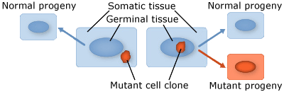
Somatic vs. Germinal Mutations
Plants are multicellular organisms, but mutation typically starts from a single cell. There are two broad categories of mutations that are classified according to the type of cell tissue involved:
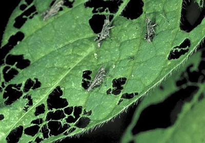
- Somatic mutations occur in somatic tissue, which does not produce gametes. Somatic cells divide by mitosis and therefore through that process, mutations can be passed on to daughter cells. Somatic mutations may have no effect on the phenotype if their function is covered by that of normal cells. However somatic cells that stimulate rapid cell division are the basis for tumors in plants and animals. Somatic mutations usually occur as single events (typically in a single cell) in multicellular organisms or organs that lead to chimera, which is a part of a plant with a genetically different constitution as compared to other parts of the same plant. Somatic mutations are not transmitted to progeny (Fig. 1).
- Germinal or germ-line mutations occur in reproductive cells that produce gametes, and therefore can be passed on to future generations. Germ cells or gametes are formed by meiosis. If a germinal mutation is inherited, then it can be carried in all of the somatic and germ-line cells of the offspring (Fig. 1).
Effects of Mutation on Fitness or Function
Mutations can affect fitness in various ways and can therefore be classified based on their effect on individual fitness:
- Deleterious mutations are those that are harmful and have a negative effect on phenotype, decreasing the fitness of the individual.
- Advantageous mutations are those that are beneficial and have a positive or desirable effect on phenotype, increasing the fitness of the individual.
- Neutral mutations have neither beneficial nor harmful effects.
- Lethal mutationsare detrimental and lead to the death of the organism when present.
Mutations can also be classified by their effect on gene function:
- Loss-of-function mutations either result in a gene product that has less function or one that has no function. Phenotypes associated with loss-of-function mutations are usually recessive. Many of the mutations that are associated with crop domestication from wild progenitors involve loss-of-function alleles (Gepts 2002).
- Gain-of-function mutations result in a gene product that has novel function. Altered phenotypes associated with gain-of-function mutations are usually dominant. Many of the changes in crop plants brought about by genetic engineering involve gain-of-function mutations (Gepts 2002).
However, it is important to underscore that not all mutations occur in genes or protein-coding regions of the chromosome, nor do all mutations that do occur in genes lead to altered proteins.
Point vs. Chromosomal Mutations
Mutations are often divided into those that affect a single gene, termed a gene mutation—also sometimes called a point mutation—and those that affect the structure of chromosomes, called a chromosomal mutation. These latter two classes of mutations will be covered in more detail after the concept of gene expression is introduced in the following section.
Point Mutation
Point or Gene Mutation
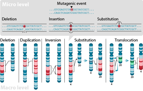
A point mutation is when a single base pair (or just a few) is altered (Fig. 2), an alteration at a “micro” level. There are two general types of point mutations: substitutions or insertions and deletions (the latter two are collectively called INDELs).
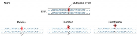
- Base pair substitutions involve an alteration of a single nucleotide in the DNA. A substitution mutation can entail either a transition or a transversion:
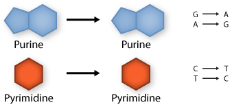
Transition: purine replaced by a different purine or pyrimidine by a different pyrimidine 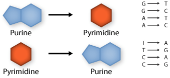
Transversion: purine replaced by a pyrimidine or pyrimidine by a purine
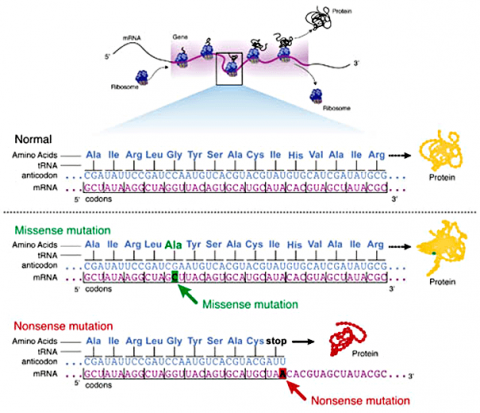
Missense Mutations
Some substitution mutations have no effect on the protein coded for. One reason is because of the redundancy of the genetic code (recall that about one fourth of all base pair substitutions code for the same amino acid; such mutations are termed silent mutations since there is no change in amino acid that results from the substitution). Another reason for lack of effect is that even if a change in amino acid occurs (termed missense mutation), it may have no actual influence on the function of a protein (Fig. 3). Also any mutation located within a non-coding region of the chromosome will not be translated into a protein. Lastly, an altered gene may be masked by other normal copies of the gene present in the genome.
In certain cases, point mutations can have a significant effect—particularly when a substitution produces a stop codon so that the alteration causes the protein synthesis to halt before the protein is entirely translated, altering the entire structure. These are called nonsense mutations (Fig. 3).
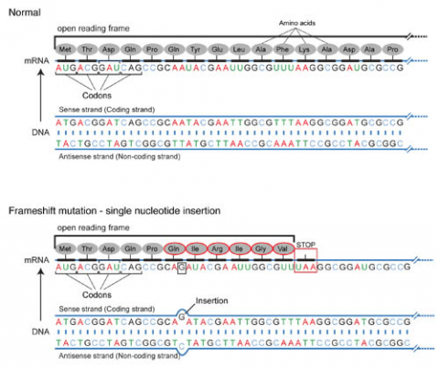
Frameshift Mutation
Base pair insertions and deletions are additions (INDELs) or losses of one to several nucleotide pairs in a gene (Fig. 2). Mutations that are insertions and deletions tend to have a much greater effect than do mutations that are base pair substitutions because they disrupt the normal reading frame of trinucleotides. Recall that each group of three bases corresponds to one of 20 different amino acids used to build a protein. Mutations involving base pair insertions and deletions are often therefore referred to as frameshift mutations. Under these circumstances the DNA sequence following the mutation is read incorrectly (Fig. 4).
Chromosomal Mutation
MUTATIONS INVOLVING CHROMOSOME SEGMENTS
Different cells of the same organism and different individuals of the same species generally have the same number of chromosomes, and homologous chromosomes are typically uniform in number and in the arrangement of genes along them. However, mutations can occur that alter the number or structure of chromosomes.
Changes involving chromosomal rearrangements entail the following basic types: deletions, duplications, insertions, inversions, substitutions, and translocations—alterations that occur at a “macro” level (Fig. 5).
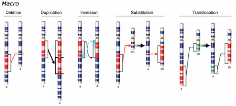
- Chromosomal deletions are when loss of a chromosome segment occurs.
- Chromosomal duplications occur when a chromosome segment is present more than once in a genome or along an individual chromosome (Fig. 5). Mutations of this type can involve duplication of chromosome fragments of either noncoding regions or genes that do code for a protein or other gene product. Gene duplications have been important events in the evolution of many crop plants, for example in cotton.Both chromosome deletions and duplications generally result from unequal crossing over during meiosis, whereby one gamete receives a chromosome with a duplicated segment or gene and the other gamete receives a chromosome with a missing or "deleted" segment.
- Chromosomal inversions happen when two breaks occur in a chromosome and the broken segment turns 180°—reversing the orientation of the sequence—and then reattaches (Fig. 5). Such inverted segments may or may not involve the centromere (termed pericentric inversion vs. paracentric inversion). A consequence of chromosomal inversions is that they either prevent crossing over or if crossing over occurs, the recombinants may be eliminated during meiosis. During meiosis, inverted chromosome segments may form loops in order to pair with the same (non-inverted) sequence on homologous chromosomes.
- Chromosomal insertions (not pictured) and chromosomal substitutions are when gain of an extra fragment of chromosome occurs (Fig. 5).
- Chromosomal translocations entail a change in the location of a chromosome segment. Commonly translocations are reciprocal and thus result from exchange of segments between two non-homologous chromosomes (Fig. 5).
Transpositions
Chromosome segments can also be translocated to a new location on the same chromosome or to a different chromosome but without reciprocal exchange; both of the latter types of mutations are termed transpositions. A transposon (also called a transposable element) is a DNA element that can move from one location to another. These mobile DNA sequences commonly occur in some genomes and can themselves cause other mutations to occur, depending on where they "transpose".
Discussion
Mutants and mutations are best known in the context of horror films. In the context of plant breeding and more generally crop production, discuss the consequences of mutations—are they good or bad? Which kinds of mutations are desirable and which ones are undesirable?
Sources of Variation
Sources of Genetic Variability
Plant breeding is dependent on differential phenotypic expression. Loci with only one allelic variant (homozygosity) in a breeding population have no effect on the phenotypic variability. Variation can be introduced to breeding populations by various methods:
- hybridization and recombination by sexual reproduction within or between species or populations
- genetic transformation or genetic engineering using recombinant DNA methods
- induced or spontaneous mutations and transposable elements (transposons)
- chromosome manipulation via change in chromosome number and structure (ploidization) [to be discussed in the module on Ploidy—Polyploidy, Aneuploidy, Haploidy]
- tissue or cell culture techniques [to be discussed in the module on Ploidy—Polyploidy, Aneuploidy, Haploidy]
CONCEPT OF CROP GENE POOLS
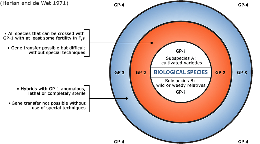
Plant germplasm is a term used to refer to an individual, group of individuals or a clone that represents a genotype, population, or species. With reference to a given crop and its wild and cultivated relatives, the concept of gene pool (all of the genes shared by individuals in a group of interbreeding individuals) has been applied to categorize a broad range of plant genetic resources according to the ease of gene transfer or gene flow to the particular crop species (Harlan and de Wet 1971).
Gene Pools
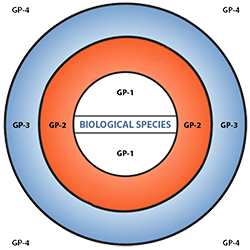
Figure 6 depicts three main categories in the original scheme outlined by J. R. Harlan and J.M.J. de Wet (1971) defined as:
- primary gene pools (GP-1, consisting of biological species that can be intercrossed easily without problems of fertility in the progeny; including both cultivated varieties and wild progenitors of the crop),
- secondary gene pools (GP-2, consisting of more distant relatives that can be intercrossed with difficulty and result in diminished fertility in the hybrids and later generations; including both cultivated and wild relatives of the crop), and
- tertiary gene pools (GP-3, consisting of very distant relatives that can be hybridized with the crop only with special techniques, e.g., embryo rescue, due to problems such as sterility, lethality and other abnormalities),
With the addition of a fourth gene pool that contains synthetic variants and lines with nucleic acid sequences that do not normally occur in nature. Methods of genetic engineering relevant to this fourth gene pool category will be covered briefly in the next section of this module. Examine a more detailed view of the gene pool concept.
Genetic Engineering
Plant Transformation
GENETIC ENGINEERING AND PLANT TRANSFORMATION
Genetic engineering, also referred to as recombinant DNA or rDNA technology or gene splicing, involves moving a DNA segment from one organism into another to 'transform' the recipient or host. Through a broad range of techniques encompassing biotechnology (for example, gene manipulation, gene transfer, cloning of organisms), novel genetic diversity can be generated that extends beyond species boundaries or can be designed and synthesized de novo in molecular laboratories. Potentially, any gene from any species, as well as synthesized segments, could be transferred into a plant using genetic engineering.
Gene transfer can be applied for a variety of objectives:
- Add different or new functions
- Alter existing traits—amplify, suppress, or prevent the expression of a gene already present in the recipient's genome
- 'Tag' and isolate genes in the recipient plant
- Tool for basic gene regulation and developmental studies
Requirements for Gene Transfer
In order to efficiently generate transformants (plants that possess DNA introduced via recombinant DNA technologies), the transformation system used must satisfy several requirements.
- Ability to get DNA into host cells in high concentration to increase the probability of incorporation into the host genome
- Incorporation into the host nucleus (or chloroplast if the objective is to minimize gene flow by pollen or to produce a large quantity of therapeutic proteins)
- Integration into host genome (or stabilization as an autonomous replicon—a plasmid or minichromosome)
- The introduced gene is expressed and translated properly
GENERAL STEPS
- Identification and isolation of a gene that confers a desired trait.
- Introduce the gene into a suitable construct and carrier, such as plasmids or bacterial vectors, for delivery into the host.
- Introduce the DNA into the host.
- Identify and select transformants.
- Regenerate plants.
- Assay for expression of the trait.
- Test for normal sexual transmission, or asexual propagation, of the transferred gene.
The carrier that will deliver the DNA into the host should have certain features.
- Sites in which to insert passenger DNA sequences (gene of interest, plus a selectable marker gene if the gene of interest does not allow for easy selection of transgenic plants).
- Sequences to mediate integration into the host genome
- Selectable marker gene for identification and selection of transformants
Usually, the DNA sequence to be transferred into the host is joined with other sequences to facilitate transfer, incorporation, and expression of the gene. Here's a generalized construct for a T-DNA vector, a carrier derived from an Agrobacterium tumefaciens plasmid (Fig. 1).
The original version of this chapter contained H5P content. You may want to remove or replace this element.
Fig. 1 Diagram of a DNA construct
Introduce the DNA
Several methods are available to introduce the DNA into the host.
- Vector-mediated transfer
- Direct DNA uptake—DNA cannot be taken directly into cells having a cell wall so protoplast must be used.
- Microinjection—DNA is injected directly into the host nucleus
- Acceleration of DNA—coated particles - particles are "shot" into the cell (particle bombardment or gene gun)
Genetic transformation plays an important role in modern-day crop improvement. The first transgenic plant was created in 1983. By 1996, there were already 1.7 million hectares of genetically modified (GM) crops and this number increased 100-fold to 170 million by 2012 and is still increasing. The majority of the GM crops (soybean, corn, cotton, papaya, canola and sugarbeet) were created by the use of Agrobacterium tumefaciens (vector-mediated transfer) to resist either herbicides or insects. Herbicide-resistant crops greatly simplified weed management where mechanization in agriculture is high. Insect-resistant crop plants produce stable yields. The tremendous expansion of GM crop production, however, is not realized without controversies. There is currently an intense public debate over the impact of GM crops on human and animal health. Besides health issues, other concerns surrounding GM crops are whether they can create superweeds by crossing to related weeds, become invasive or cause unintended harm to wildlife.
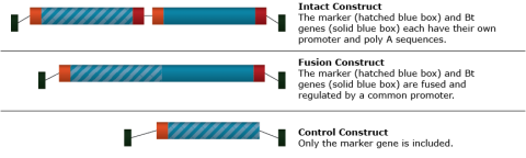
Bt Gene: Vector Constructs
Let's follow the transfer of a Bt gene into a plant.
The Bt gene was identified and isolated from Bacillus thuringiensis, a bacterium. The gene produces a protein that has toxic effects on Diptera (flies), Lepidoptera (butterflies and moths), and Coleoptera (beetles) species. Soybean was transformed using Agrobacterium tumefaciens. Two different T-DNA vector constructs carrying the Bt gene and one control construct were tested for effectiveness in transforming soybean cells and expressing the Bt toxin (Fig. 7).
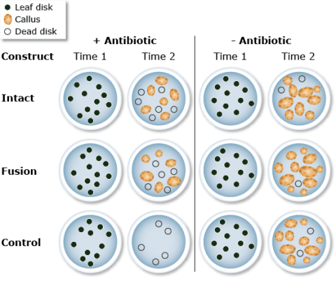
Bt Gene: Transformation
Leaf disks from soybean plants were infected and cultured on selective (+) and control (-) media—the selective medium was gradually enriched with an antibiotic (Fig. 8). At time 1, the leaf disks were infected with the respective constructs. Conditions were used to promote callus production and growth. At time 2, the plates were evaluated for calli formation.
The original version of this chapter contained H5P content. You may want to remove or replace this element.
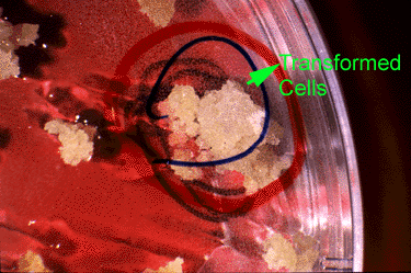
Transformed cells are able to develop into calli. These are selected and transferred to a medium containing both antibiotics and growth regulators that promote the formation of shoots and roots (Fig. 9).
Bt Gene: Insect Resistance Evaluation
Plantlets are regenerated and transferred to pots containing sterilized soil. Nearly all of the regenerated plants exhibited normal morphology and vigor. A few had chlorophyll deficiencies— these were eliminated from the study. The remaining regenerated plants were evaluated for insect resistance. An equal number of insect larvae are placed on each regenerated plant; plants are isolated to prevent insects from moving among plants.
Bt Gene: Insect Resistance Data Analysis
After several days, the dead larvae on each plant are counted. Here are the data.
| Gene Construct | No. of Plants Showing % Larvae Mortality | |||
| < 25 % | 25% - 50% | 51% - 75% | 76% - 100% | |
| Intact | 14 | 7 | 0 | 0 |
| Fusion | 2 | 6 | 2 | 20 |
| Control | 29 | 0 | 0 | 0 |
Study the information in the above table. Look for any patterns in the data. Interpret the data by selecting all of the true statements
The original version of this chapter contained H5P content. You may want to remove or replace this element.
Advantages and Disadvantages
Although recombinant DNA technologies have some problems, the technologies offer several advantages.
| Advantages | Disadvantages |
|---|---|
| Characters can be transferred from divergent species without the limitation of sexual compatibility | Difficult to identify and isolate gene |
| Single gene or gene sets can be transferred into important breeding lines without the deleterious effects of linked genes. | Insertion is random |
| Transferred character ordinarily exhibits dominant, single-gene inheritance | Difficult to obtain proper expression |
| Still must screen at whole plant level and under normal production conditions | |
| Expensive |
Despite its limitations, plant transformation has additional advantages over conventional breeding. Millions of cells, with regeneration capacity, can be screened for the desired trait in a few weeks. A desired gene can be transferred without the necessity of generations of breeding to move the trait from one line into another. Recombinant DNA technology can also be used to place synthetic genes into plant genomes.
The insertion point of the transferred gene cannot be controlled. Plants contain an estimated 500,000 to 5,000,000 kilobases (kb) of DNA. The maize genome, for example, has more than 4,000,000 kb. Generally, transferred DNA involves relatively small amounts of DNA, on the order of 10 kb, so the insertion ordinarily has little effect on chromosome pairing, recombination, or mitosis. The incorporated gene may or may not affect other genes in the recipient genome, depending on where it inserts.
- In a non-coding region—no effect on the recipient genome
- In a gene that occurs in multiple copies in the genome—the effect, if any, is usually not detectable.
- In a single-copy gene—inactivates or alters the expression of the single-copy gene.
Insertion into a single copy gene is rare. If it does insert into a single-copy gene, inactivation or alteration of the expression of the disrupted gene may be undetected, or may cause favorable or adverse results—albino and other chlorophyll deficiencies are common problems.
Why do these characters generally exhibit dominant, single-gene inheritance? Traits acquired via gene transfer often add a function to the transformed plant. Because the transferred trait is unique in the transformant's genome, the transformant does not possess any contrasting alleles for the character. Thus, its inheritance is expected to be dominant and as a single gene.
The original version of this chapter contained H5P content. You may want to remove or replace this element.
Gene transfer is also used to suppress or eliminate, or to amplify the expression of genes already possessed by the host plant. These are also usually designed to behave as dominants.
Expression involves many steps, all of which must occur properly to obtain the desired phenotype. Expression must be appropriately regulated.
- Generation of the gene's product-requires proper transcription, mRNA processing, and translation.
- Location of expression must be in the appropriate plant part.
- Timing of expression needs to occur at the right stage of the plant's development.
- Amount needs to be at an effective level or extent of expression to generate the desired phenotype.
Reflection
The Module Reflection appears as the last "task" in each module. The purpose of the Reflection is to enhance your learning and information retention. The questions are designed to help you reflect on the module and obtain instructor feedback on your learning. Submit your answers to the following questions to your instructor.
- In your own words, write a short summary (< 150 words) for this module.
- What is the most valuable concept that you learned from the module? Why is this conceptvaluable to you?
- What concepts in the module are still unclear/the least clear to you?
References
Collard, B.C.Y., M.Z.Z. Jahufer, J.B. Brouwer, and E.C.K. Pang. 2005. An introduction to markers, quantitative trait loci (QTL) mapping and marker-assisted selection for crop improvement: the basic concepts. Euphytica 142: 169-196.
Falconer, D.S. and T.F.C. Mackay. 1996. Introduction to Quantitative Genetics. 4th edition. Longman Pub. Group, Essex, England.
Harlan, J.R., and J.M.J de Wet. 1971. Towards a rational classification of cultivated plants. Taxon 20: 509-517.
Gepts, P. 2002. A comparison between crop domestication, classical plant breeding, and genetic engineering. Crop Science 42: 1780-1790.
Nageswara-Rao, M. and J.R. Soneji. 2008. Molecular genetic markers: what? why? which one for exploring genetic diversity? Perspectives-The Science Advisory Board, 8 September 2008 [available online September 23, 2011, http://www.scienceboard.net/community/perspectives.210.html].
Neuffer, M.G, E.H. Coe, and S.R. Wessler. 1997. Mutants of Maize. Cold Springs Harbor Laboratory Press.
NIH-NHGRI (National Institutes of Health. National Human Genome Research Institute). 2011. Talking Glossary of Genetic Terms. [available online February 6, 2017, http://www.genome.gov/glossary/].
For Your Information
Amino acids are the building blocks of polypeptides, proteins, and enzymes. The order of the nucleotides on a strand of RNA, as transcribed from DNA, determines the order of amino acids in a polypeptide. Each group of three consecutive nucleotides of the RNA codes for a particular amino acid, or the beginning or end of the message. These triplets of nucleotides are called codons (Fig. 20).
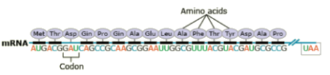
The genetic code, or instructions from a gene that direct the cell to make a specific protein, is usually based on the messenger RNA (mRNA) sequence (Fig. 21). In mRNA, uracil (U), rather than thymine (T), is the nucleotide base that complements adenine (A) on the DNA strand; guanine (G) complements cytosine (C) in both DNA and RNA.
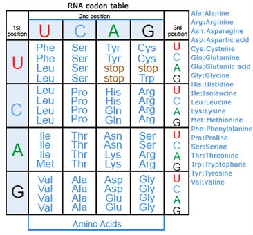
Here are some examples of codons:
- A-A-A and A-A-G signal the amino acid lysine (Lys)
- G-A-A and G-A-G code for glutamine (Gln)
- A-U-G signals the start of a coding sequencing and codes for methionine (Met)
- U-A-A, U-A-G, and U-G-A are stop codons.
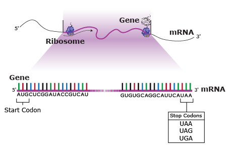
Of the 64 possible combinations of three bases, 61 specify an amino acid, while the remaining three combinations are stop codons, or trinucleotide sequences that indicate the end of the message, terminate translation of that mRNA section, and signal a “stop” to protein synthesis (Fig. 22).
The portion of a DNA molecule that, when translated into amino acids, contains no stop codons is referred to as an open reading frame (Fig. 23).
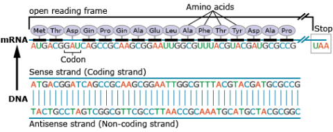
Acknowledgements
This module was developed as part of the Bill & Melinda Gates Foundation Contract No. 24576 for Plant Breeding E-Learning in Africa.
Crop Genetics, Mutations and Variation - Authors: Laura Merrick, Arden Campbell, Deborah Muenchrath, and Shui-Zhang Fei (ISU)
Multimedia Developers: Gretchen Anderson, Todd Hartnell, and Andy Rohrback (ISU)
How to cite this module: Merrick, L., A. Campbell, D. Muenchrath, and S. Fei. 2016. Mutations and Variation. In Crop Genetics, interactive e-learning courseware. Plant Breeding E-Learning in Africa. Retrieved from https://pbea.agron.iastate.edu
(1) Identical alleles are present at a locus on homologous chromosomes in a diploid or polyploid individual, such as AA in a diploid or AAAA in a tetraploid.
(2) Individual plants have identical alleles at each locus.
A localized group of actively dividing cells from which permanent specialized tissues differentiate.
