
Chapter 5: Linkage
Thomas Lübberstedt; Arden Campbell; Deborah Muenchrath; Laura Merrick; Shui-Zhang Fei; and Walter Suza
Introduction
Genes located on the same chromosome are genetically linked. Genetic linkage analysis can be used to determine the order of genes on chromosomes. Closely linked genes are not segregating independently, like genes located on different chromosomes. This has different implications, e.g., in relation to trait correlations. Moreover, linked genes can be used as genetic markers, which have become an important tool in plant breeding.
- Develop an understanding of the genetic basis of linkage.
- Gain awareness on how to detect the occurrence of linkage.
- Review the principles of genetic map construction.
- Become familiar with the concept of linkage disequilibrium.
Crossover and Recombination
Genetic Organization
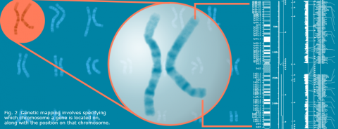
Genes are physically organized on chromosomes. Each gene is located at a particular “address” (particular position on a specific chromosome, which can be identified by genetic mapping). Inheritance of genes located on different chromosomes follows the rules of independent assortment. Since plant species have multiple chromosomes, independent assortment is true for the majority of genes. In contrast, linked genes located on the same chromosome are more likely to cosegregate, i.e., being jointly transmitted to offspring more often than expected by independent assortment. The biological process that separates linked genes is the crossing-over (C.O., or crossover), which occurs during meiosis, and leads to genetic recombination.
Crossing-Over
During meiosis of diploid organisms, the chromatids of homologous chromosomes pair and form bivalents. During Meiosis I, homologous chromatids pair to physically exchange chromosome segments. The chromosomal site, where this reciprocal exchange of homologous chromosome segments takes place, is called a chiasma. Thus, crossing-over involves not completely understood mechanisms for identification of homologous sites of chromatids, breakage and rejoining of chromosomes.
Genetic Distance
Crossing-over events occur more or less random during meiosis. In most plant species, one to few crossing-over events occur per meiosis and chromosome. Thus, the closer the genes are physically linked on the same chromosome, the less likely they will get separated, and consequently, the less likely genetically recombinant gametes will be produced. This is the underlying principle of genetic maps: the genetic distance between genes reflects the probability of a crossing-over between linked genes.
Recombination
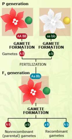
Observation of crossing-over events requires cytological methods, which can be cumbersome for large populations. In contrast, genetic recombinants can be observed at the phenotype level, or by use of DNA markers. If two linked genes with two alleles each have clear phenotypic effects, e.g., on flower color (A: red, a: white; A is dominant over a) and seed color (B: green, b: yellow; B is dominant over b), then genetic recombinants can easily be identified by determining the fraction of non-parental gametes in the offspring.
Note that crossing-over also takes place in meiosis of completely homozygous individuals. However, in this case, genetic recombination cannot be observed as described above. The reason is that observation of recombinant gametes requires two (or more) different alleles at the loci, for which linkage is going to be determined. This explains why offspring saved from pure line cultivars will not segregate whereas seed harvested from F1 hybrid will segregate. The observable fraction of recombination events is also called effective recombination.
Linkage Detection
Linkage Phase
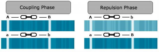
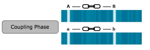
For linkage detection, it is crucial to know the linkage phase of alleles.
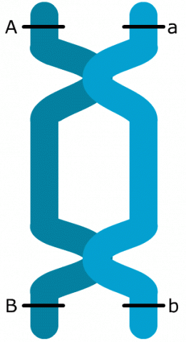
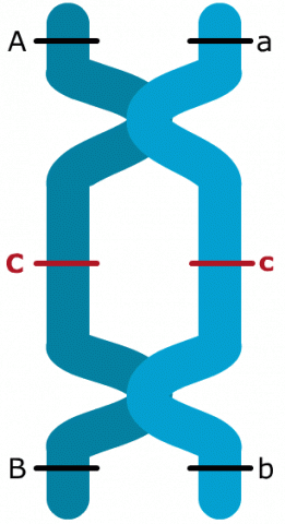
The linkage phase is the physical arrangement of linked genes in a chromosome. A double heterozygote with a genotype of AaBb could be in one of the two linkage phases. Conventionally, when linked dominant alleles are located on the same homologous chromosome and the linked recessive alleles are on the other homologous chromosome, for example, AB/ab, it is said the genes are linked in the coupling phase. When a dominant allele at one locus is on the same homologous chromosome as a recessive allele of the other linked gene, for example, Ab/aB, it is said that the genes are linked in repulsion phase (Fig. 4).
This knowledge is crucial, as linkage detection and distance estimation is based on the observed parental and non-parental gametes.
Coupling and Repulsion
In the case of close linkage, non-parental gametes and respective offspring are underrepresented.
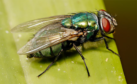
An example is the Australian sheep blowfly, Lucilia cuprina. Normal blowflies have a green thorax and surround themselves in a brown cocoon during their pupal stage. However, recessive genes (here marked a and b) can cause the fly to develop a purple thorax and spin a black puparium.
Using Testcrosses
For detection of linkage, appropriate testcrosses need to be conducted. The linkage phase is known, if two homozygous parental genotypes (AABB and aabb) are crossed to produce the respective F1 (AaBb).
In this case, A and B as well as a and b are linked in coupling phase.
The non-parental recombinant gametes have the genotype Ab and aB, whereas the parental gametes have the genotype AB and ab.
Usually the phenotype cannot be observed in (haploid) gametes, but only in diploid plants. Thus, to determine whether two loci are linked, offspring need to be produced. This can be achieved by self pollination of the AaBb – F1, by production of doubled haploid offspring, or by a testcross.
In this particular example, a backcross (BC) of the F1 to the aabb parent would be the best option.
Testcross Gametes
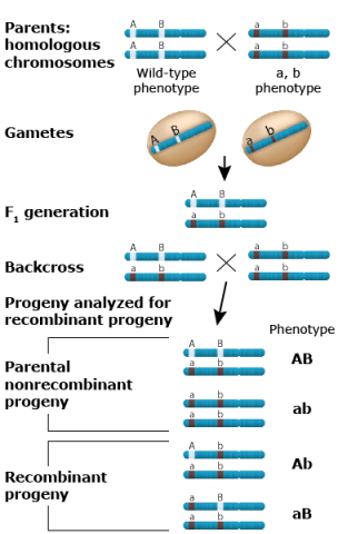
All offspring from this BC would receive an ab gamete from the aabb parent, and any of the two parental (AB, ab) or non-parental (Ab, aB) gametes from the F1.
Because of dominance of A over a and B over b, all four resulting diploid genotypes in the BC1 (backcross generation 1) generation (AaBb, Aabb, aaBb, aabb) can be phenotypically discriminated, and used to count genotypes that received parental or non-parental gametes from the F1.
Thus, when using this BC approach, only the crossing-over events that occurred in the F1 are monitored for linkage estimation.
Chi-Square Test
For detection of linkage, a Chi-Square test can be employed. The Chi-Square test compares observed with expected frequencies. In this case, the null hypothesis to determine expected frequencies is the assumption of independent assortment. Under this assumption, equal frequencies of all four gametes are expected. In the case of linkage, BC1 individuals carrying non-parental gametes are underrepresented, leading to a statistically significant Chi-Square value. This means that the null hypothesis of independent assortment would be rejected and linkage assumed.
| Phenotypes | Observed Number (o) | Expected Number (e) | d (o – e) |
d2 | d2 / e |
|---|---|---|---|---|---|
| Parentals:
(black-bodied and normal wing plus grey-bodied, vestigial wing) |
2,712 | 1,618 | 1,094 | 1,196,836 | 739.7 |
| Recombinants:
(black-bodied and vestigial wing plus grey-bodied and normal wing) |
524 | 1,618 | 1,094 | 1,196,836 | 739.7 |
Chi-Square Results
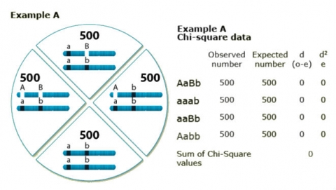
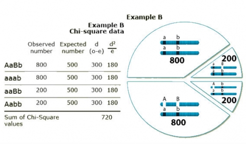
To better understand the use of Chi-Square in determining linkage, two numerical examples based on the cross schemes described in Figs. 8 and 9 are provided here. In both examples, a sample size of 2,000 BC1 individuals has been used.
The Chi-Square test sums up over all squared differences between observed and expected values, divided by expected values.
In example A, observed and expected values are equal, thus the Chi-Square value = 0.
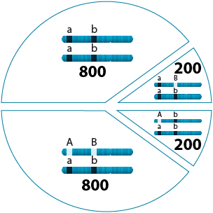
In example B, the squared differences between observed and expected values is in all cases 90,000, to be divided by the expected 500 = 180. As there are four genotypic classes, the Chi-Square value is 720, which is significantly larger than the tabulated value of 3.81 (p = 5%).
In conclusion, example A is in agreement with independent assortment, whereas in example B, linkage has been detected.
In conclusion, example A is in agreement with independent assortment, whereas in example B, linkage has been detected.
Genetic Distance
400 / 2000 = 0.2
0.2 x 100% = 20%
The same data used to determine linkage can also be used to estimate the recombination frequency between two genes (more precisely, the recombinant frequency). The recombinant frequency = (number of BC1 progeny with recombinant (non-parental) alleles / total number of BC1 progeny) x 100%.
In example B of Section 2: Linkage Detection, the recombinant frequency is (200 + 200 / 2000) * 100% = 20%.
The recombination frequencies between any pairs of genes provide an estimate of how close they are linked on a chromosome. The recombinant frequency in % is sometimes also called “map units” (M.U.). In this example, the genetic distance in map units between the two genes under consideration is 20 M.U.
In the case of complete linkage of two genes, no recombinants would be expected. The recombinant frequency would be 0%, which represents the lower limit of recombinant frequencies.
In the case of random segregation, the expected numbers of recombinant and nonrecombinant alleles are equal. Thus, the upper limit of recombinant frequencies in the case of unlinked or loosely linked genes is 50%.
Even for gene pairs located at the different ends of the same chromosome, recombination frequency can reach 50%. The procedure to determine recombination frequencies between any pair of genes is called two-point analysis.
You have a F1 plant heterozygous at two loci that are 12 map units apart on the same chromosome. The F1 received linked recessive alleles from one parent and linked dominant alleles from the other parent.
You have a F1 plant heterozygous at two loci that are 12 map units apart on the same chromosome. The F1 received linked recessive alleles from one parent and linked dominant alleles from the other parent.
Since linkage cannot be detected in the F1, you self-pollinate the F1 and evaluate the F2. What would be the F2 and testcross percentages if the F1 percentages in the case of repulsion phase of the recessive alleles?
Three-Point Analysis
Purpose
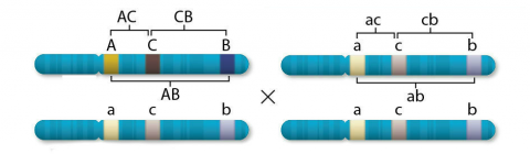
Whereas two-point testcrosses establish linkage between pairs of genes, three-point testcrosses facilitate establishment of the order of genes on chromosomes, as a prerequisite to establishing genetic maps. If a third locus with alleles C and c (C is dominant over c) is added to the case mentioned in Genetic Distance, where A and B are linked in coupling phase and the dominant allele C is in coupling with A and B, then eight different testcross progeny would result from a backcross with the recessive parent.
| Class | Genotype of gamete from heterozygous parent | Number | Origins | |||
|---|---|---|---|---|---|---|
| 1 | A | C | B | 179 | } | Parentals, no crossover |
| 2 | a | c | b | 173 | ||
| 3 | A | c | b | 52 | } | Recombinants, single crossover AC |
| 4 | a | C | B | 46 | ||
| 5 | A | C | b | 22 | } | Recombinants, single crossover CB |
| 6 | a | c | B | 22 | ||
| 7 | A | c | B | 4 | } | Recombinants, double crossover AC, CB |
| 8 | a | C | b | 2 | ||
Frequency Chart
Pairwise recombination frequencies can be determined as described in the chart.
- 20.8% for AC (AC recombinants are in classes 3, 4, 7, and 8; thus, the recombination rate between A and C is (52+46+4+2/500) * 100% = 20.8%)
- 10% for CB (CB recombinants are in classes 5-8)
- 28.4% for AB (AB recombinants are in classes 3-6).
Once linkage between pairs of three (or more) genes has been established, the next question is how they are arranged in linear order on chromosomes, which could be ABC, ACB, or CAB.
| Class | Genotype of gamete from heterozygous parent | Number | Origins | |||
|---|---|---|---|---|---|---|
| 1 | A | C | B | 179 | } | Parentals, no crossover |
| 2 | a | c | b | 173 | ||
| 3 | A | c | b | 52 | } | Recombinants, single crossover AC |
| 4 | a | C | B | 46 | ||
| 5 | A | C | b | 22 | } | Recombinants, single crossover CB |
| 6 | a | c | B | 22 | ||
| 7 | A | c | B | 4 | } | Recombinants, double crossover AC, CB |
| 8 | a | C | b | 2 | ||
Gene Order
The most likely gene order minimizes the sum of pairwise recombination frequencies within a three-gene interval, which would be:
- 38.4 for ABC (28.4% for AB + 10% for CB)
- 30.8 for ACB (20.8% for AC + 10% for CB)
- 49.2 for CAB (20.8% for AC + 28.4% for AB)
Thus, the most likely gene order is ACB. In other words, the interval between A and B can be subdivided into the intervals between AC and CB.
| Class | Genotype of gamete from heterozygous parent | Number | Origins | |||
|---|---|---|---|---|---|---|
| 1 | A | C | B | 179 | } | Parentals, no crossover |
| 2 | a | c | b | 173 | ||
| 3 | A | c | b | 52 | } | Recombinants, single crossover AC |
| 4 | a | C | B | 46 | ||
| 5 | A | C | b | 22 | } | Recombinants, single crossover CB |
| 6 | a | c | B | 22 | ||
| 7 | A | c | B | 4 | } | Recombinants, double crossover AC, CB |
| 8 | a | C | b | 2 | ||
Expressed yet another way: incorrectly ordered genes would increase the total map length because part of the recombination events would be counted twice. If ACB is the true order, then the genetic length of, e.g., ABC would be inflated, because recombinants for the segment BC would be counted two times: for the interval BC, in addition to the same interval within the segment A(C)B. Algorithms of mapping programs use this principle (minimizing the genetic distance) for three-point analyses.
Double Crossovers
The two-point recombination frequency between A and B (28.4%) differs from the sum of recombination frequencies for AC and CB (30.8%). The reason for this discrepancy is the occurrence of double crossover events. These are two crossovers in a single meiosis within an interval of interest and the second crossover reverses the effect of the first crossover, i.e., the second crossover returns the B allele to the original position before the first crossover. For this reason, by only taking recombinants between A and B into consideration, double crossovers cannot be observed. Because a double crossover exchanges chromosome segments within an interval of two genes, the linkage phase (coupling) of those two genes remains unchanged.
Observing Double Crossovers
Only by adding a gene like C in between A and B, it is possible to observe double crossovers. In the case of the interval between genes A and B, six double crossovers were observed. In consequence, recombination and crossover frequencies are not identical. The larger the genetic interval, the larger the discrepancy between recombination and crossover frequencies, because even-numbered crossover events within a pair of genes go undetected. By adding an additional gene in this interval, at least some double crossovers can be detected. This leads to detection of additional recombination events. For this reason, the recombination frequency between A and B in the example is increased, after adding C in between those two genes, because 6 double crossovers (= 12 additional recombination events) could be detected. Those 12 additional detectable recombination events explain for the 2.4% difference between recombination frequencies detected for the gene pair A and B with or without inclusion of C.
Phase Analysis
Recombinants resulting from double crossovers are always in the lowest frequency (class 7 and 8, respectively in this table). To determine which allele is in the middle, a convenient method is to find out which allele in the double crossover recombinants has changed its linkage phase with the other parental alleles (in classes 7 and 8, allele C/c has changed its linkage phase with the other alleles).
| Class | Genotype of gamete from heterozygous parent | Number | Origins | |||
|---|---|---|---|---|---|---|
| 1 | A | C | B | 179 | } | Parentals, no crossover |
| 2 | a | c | b | 173 | ||
| 3 | A | c | b | 52 | } | Recombinants, single crossover AC |
| 4 | a | C | B | 46 | ||
| 5 | A | C | b | 22 | } | Recombinants, single crossover CB |
| 6 | a | c | B | 22 | ||
| 7 | A | c | B | 4 | } | Recombinants, double crossover AC, CB |
| 8 | a | C | b | 2 | ||
Coefficient of Coincidence and Interference
Crossover events in adjacent chromosome regions might affect each other, a phenomenon called interference. Most typically, a crossover event in one region tends to suppress a crossover in the adjacent regions. The extent of interference is expressed by the coefficient of coincidence, which is equal to the observed frequency of double crossovers / expected frequency of double crossovers.
| Class | Genotype of gamete from heterozygous parent | Number | Origins | |||
|---|---|---|---|---|---|---|
| 1 | A | C | B | 179 | } | Parentals, no crossover |
| 2 | a | c | b | 173 | ||
| 3 | A | c | b | 52 | } | Recombinants, single crossover AC |
| 4 | a | C | B | 46 | ||
| 5 | A | C | b | 22 | } | Recombinants, single crossover CB |
| 6 | a | c | B | 22 | ||
| 7 | A | c | B | 4 | } | Recombinants, double crossover AC, CB |
| 8 | a | C | b | 2 | ||
The expected frequency of double crossovers is the product of two single crossovers in adjacent regions assuming there is no interference.
In this example, this expected frequency is 0.21 (recombination frequency for AC) * 0.10 (recombination frequency for CB) = 0.021.
The observed frequency of double crossover events is 6/500 in the example, resulting in 0.012. Thus, the coefficient of coincidence in this example is 0.012/0.021 = 0.58.
Interference is defined as 1 − coefficient of coincidence, which would be 0.42 in this example. A value of zero for interference would mean that a crossover in one region does not affect crossovers in the adjacent region. Interference of 1 means, that crossovers in one region suppress crossovers in the adjacent region. Negative values are possible and have been reported in some instances, which means that crossovers in one region stimulate crossovers in the adjacent region.
Map Functions
Measurement Units
The purpose of genetic maps is to report the length of chromosome intervals, chromosomes, and whole genomes. Since recombination frequencies converge to a value of 50% as reported above, indicating the absence of linkage, recombination frequencies are not additive and, thus, not useful to describe the distance between genes that are located far apart. When recombination frequency reaches 50%, it would be impossible to tell whether the genes are located far apart on the same chromosome or on different chromosomes.
Instead, estimates of the number of crossover events are used as an additive measure of genetic map distances. The unit for measuring genetic distances is Morgan (M), or usually centiMorgan (cM). In contrast to recombination frequencies, map units expressed in cM are additive. One Morgan reflects the observation of one crossover event per single meiosis. One cM is a distance between genes that produces 1% recombinants in the offspring. Typical lengths of genetic maps in maize, for example, vary between 1,600 to 2,000 cM, which means that on average, 1.6 – 2 crossovers occur per chromosome and single meiosis in maize (maize has 10 homologous chromosome pairs).
Frequency Conversion
As mentioned above, direct observation of crossover events is cumbersome. For that reason, most genetic maps published to date are based on the conversion of recombination frequencies into crossover frequencies. The main obstacle to translating recombination frequencies into crossover frequencies is the variable and unknown degree of interference in different genome regions. While it has been possible in the earlier example to determine the degree of interference, and thus frequency, of double crossover events, in the genetic interval between A and B by adding C, the degree of interference between AC and CB is unknown. This could be addressed by observing segregation of further genes within these two regions (if available), but this issue could ultimately only be addressed by complete genome sequencing of all offspring in a mapping population, which at this point is still too costly.
Visual Relationship
Instead, map functions have been developed, that translate recombination frequencies into crossover frequencies, and thus cM (see Fig. 14 below). Figure 14 clearly shows, that there is an approximately linear relationship between recombination rates (y-axis) and crossover rates (x-axis). However, with increasing map distances, recombination rates converge to 50%. In other words, gene pairs with crossover rates of 80 cM or 200 cM, respectively, would be nearly indistinguishable based on recombination rates, which would result in recombination rates between 40 and 50%.
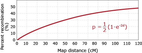
The various available map functions make different assumptions on the extent of interference. For example, the Haldane mapping function assumes absence of interference. In contrast, the Kosambi function assumes the presence of interference.
Other Types of Maps
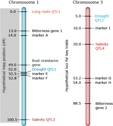
Genetic maps can be generated in other ways than using testcrosses. Examples include somatic cell hybridization and tetrad analysis. In plants, interspecies addition lines such as oat-maize addition lines created by distant hybridization have been developed as tool for mapping of genes. If two genes appear on the same addition segment, they are genetically linked. Besides genetic maps, cytological and physical maps can be established.
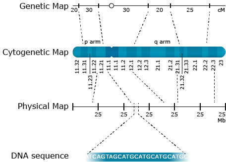
Cytological maps show gene orders along each chromosome as determined by cytological methods whereas physical maps are measured in base pairs as determined by DNA sequencing. With rapid progress in sequencing technology and an increasing number of sequenced plant genomes, physical maps gain in importance. Complex plant genomes like the maize genome are billions of base pairs long. When comparing genetic and physical maps, the order of genes is conserved. However, the relative distances between genetic and physical maps might vary substantially. The reason is that crossover events are not evenly distributed in genomes. Usually, crossover events tend to be suppressed in centromere and repetitive DNA regions, whereas they are enhanced in gene-rich regions.
Cytogenic Map
Factors Influencing Linkage Mapping
Linkage mapping based on testcrosses can be affected by selection or incomplete penetrance, among others. Selection in the most extreme case would be due to lethality of gametes (gametic selection) or zygotes (zygotic selection). If a backcross is used for linkage detection, as described above, lethality of male gametes carrying for example the a allele would lead to only two classes of BC progeny, if AaBb is crossed as pollinator to aabb. In that case, only AaBb (parental) and Aabb (recombinant) genotypes would be obtained. Zygotic selection affects the viability of particular genotypes. If the aa genotype in the example above is lethal, then the aa offspring derived from self-pollination of an AaBb genotype would be missing. Incomplete penetrance means that a genotype that is supposed to express, for example, red flowers, has to a certain extent white flowers. In other words, there is no 100% match between genotype and phenotype, but due to environmental factors, the phenotype might differ. As for selection, incomplete penetrance alters the frequency of expected genotypes in testcrosses, which is the basis for detection of linkage.
Consequences and Applications of Linkage
The main application of linkage is in genetic mapping of genes using molecular markers. Once genes have been mapped and closely-linked markers identified, those markers can be used for marker-aided selection procedures. Technological progress in DNA methods has been and still is rapid, so that thousands of markers can be produced at low cost in any species of interest. Moreover, novel genomic selection strategies addressing complex inherited traits are being developed.
Linkage can in some cases be confused with pleiotropy. If a favorable character (e.g. resistance) is always inherited together with an unfavorable trait (e.g., lodging), a negative pleiotropic effect might be assumed, which might alternatively be caused by two closely linked genes. Whereas close linkage can be resolved to find favorable genotypes for both traits, this is not true for pleiotropy. Linkage reduces the possible genetic variation in small populations. With increasing numbers of generations, or population sizes, genetic variation can be increased. Similarly, inbreeding reduces the opportunity for effective recombination.
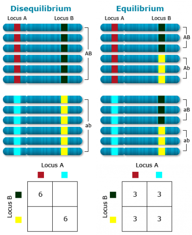
Linkage Disequilibrium
Genotype Distribution
Although allele frequencies at individual loci are expected to be stable in the case of random mating, genotype frequencies at two or more loci jointly do not achieve this equilibrium after one generation of random mating.
To illustrate this point, consider two populations, one consisting of entirely AABB genotypes and the other consisting entirely of aabb genotypes. Assumed they are mixed equally and allowed to randomly mate. The first generation would consist of the three genotypes AABB, AaBb, and aabb in the proportions 1/4 : 1/2 : 1/4. However, for two loci, each with two alleles, nine genotypes are possible. (For n alleles at each locus and k loci, there are: [latex](\frac{n(n+1)}{2})^k[/latex] possible genotypes). Continued random mating would produce the missing genotypes, but they would not appear at the equilibrium frequencies immediately.
Equilibrium
Consider the following examples based on two alleles at each of two loci:
- Alleles: A a B b
- Allele frequencies: PA Pa PB Pb
- Gametic Types: AB Ab aB ab
- Gametic Frequencies: PAB PAb PaB Pab
In linkage equilibrium, the expected gamete frequencies can be calculated from the marginal allele frequencies. For example, in equilibrium, the frequency of gamete AB (PAB) would be expected to be equal to the product of the frequencies of the A allele (PA) and the B allele (PB).
This is valid under the following conditions: PA + Pa = 1; PB + Pb = 1; and PAB + PAb + PaB + Pab = 1.
If, for example, the allele frequencies of PA = Pa and PB = Pb are 0.5, then the frequencies of all gametes are 0.25.
A measure for Disequilibrium, D = PAB – PA*PB. D = 0 in the case of equilibrium. If D differs from 0, it reflects presence of Disequilibrium. In other words, the frequency of a gamete differs from its expected frequency based on marginal probabilities of the respective individual alleles.
LD and Mapping
Linkage disequilibrium is the non-random association of alleles at different loci. LD is extensively used in mapping human disease genes using natural populations (Association mapping).
In plants, gene mapping has been conducted mainly by using mapping families because of the ease with which mapping families are created, but LD mapping using natural populations is increasing rapidly because such populations are large in size and have much greater allelic diversity.
LD Statistic D’
|D’| = [latex]\dfrac{D^2_{AB}}{min (p_Ap_b,p_Ap_b)}[/latex]
for DAB < 0
|D’| = [latex]\dfrac{D^2_{AB}}{min (p_Ap_b,p_Ap_B)}[/latex]
for DAB > 0
Dissipation
It can be shown that after t generations of random mating, the remaining disequilibrium is given by:
[latex]D_t = D_0 (1 - c)^t[/latex]
where, D0 is the disequilibrium in generation 0 and c is the recombination fraction, with c = 0.5 for independently segregating loci, which is identical to a recombination frequency of 50% (the range of c is from 0 to 0.5, whereas the range of r is from 0% to 50%). The dissipation of disequilibrium relative to generation 0 is given in Fig. 18.
Recombination and LD
Generally, deviations from independence at multiple loci are referred to as linkage disequilibrium, even if genetic linkage is not the cause (in other words, alleles are not physically linked). Unless two loci are known to reside on the same chromosome, the term Gametic Disequilibrium should be used to describe disequilibrium among loci. Whereas recombination and crossover frequencies, as mentioned initially, are used to describe the distance between genes from a chromosomal perspective, linkage disequilibrium is mostly used to describe a property of populations. However, both terms are closely related.
Genetic Markers
Overview
Genetic variation results from differences in DNA sequences and, within a population, occurs when there is more than one allele present at a given locus. Such populations are referred to as populations that are polymorphic or segregating at that locus. The opposite situation is when all members of the population are homozygous for the same allele, in which case the population is said to be fixed or monomorphic for that allele. A genetic marker is a DNA sequence that exhibits polymorphism among individuals and can thus be used to identify a particular locus (although not necessarily a gene) on a particular chromosome; the marker itself may be part of a gene or may have no known function. Markers are inherited in a Mendelian fashion and facilitate the study of inheritance of a trait or sometimes a linked gene. Markers are used to identify, map, and isolate genes, select desired genotypes, and detect genetic variation or determine genetic relationships among individuals. Markers are regions of genomes that are heritable, often easy to document, and useful for detecting genetic variation.
Three Types
Genetic markers generally do not represent target genes of interest to a breeding program, but instead are useful as ‘signs’ or ‘tags’, particularly when they are closely linked to genes that control a trait of interest. A genetic map constructed with genetic markers is similar to a road map. Linkage groups in a genetic map represent roads whereas individual markers on each linkage group represent signs or landmarks that help plant breeders to navigate through the plant genome and find the genes of interest.
There are three major categories of markers.
- Morphological markers
- Biochemical markers
- Molecular markers
Morphological Markers
These types of markers (also called visible or classical markers) are phenotypic traits with only a few distinct morphs or variants (e.g., flower color or seed shape), usually due to one or perhaps two gene loci so they are not strongly affected by the environment. Inheritance patterns of visible and morphological characters have been used to map genes to particular chromosome segments and to identify linkage groups. Such markers are limited in number compared to the abundance of DNA markers, however, and may be influenced by developmental stage of the plant.
Biological Markers
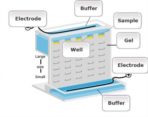
Isozymes (sometimes called allozymes) are allelic variants of a single enzyme that share the same function, but may differ in level of activity due to differences in amino acid sequence. Isozymes are proteins for which variation can be detected by differential separation using electrophoresis, a technique for separating macromolecules (DNA, RNA, protein) on a gel by means of an electric field and specific chemical staining.
Isozymes have codominant expression, meaning that both homozygotes can be distinguished from the heterozygote and neither allele is recessive. In contrast to codominant markers, dominant markers are either present or absent.
In comparison to visible polymorphisms, they reveal more of the underlying genetic variation. However isozymes are gene products, so they reveal only a small subset of the actual variation in DNA sequences between individuals and do not reveal variation in the non-coding regions of the genome. In general, such markers are limited in number and have limited use in genetic mapping studies.
Molecular Markers
Molecular or DNA markers reveal sites of variation in DNA. Variability in DNA facilitates finer scale mapping and detection. Mapping is the process of making a representative diagram cataloging genes and other features of a chromosome and showing their relative positions. Many of these molecular markers avoid the limitations associated with visible and biochemical markers. They facilitate the evaluation of genome-wide coverage and are not affected by environmental factors or developmental stages. They allow high resolution of genetic diversity to be detected. Molecular markers have added substantial amounts of information to our genetic maps.
Any DNA sequence can be genetically mapped, like genes leading to plant phenotypes as long as there is a polymorphism available for the sequence to be mapped, i.e., two or more different alleles. This can basically be a single nucleotide polymorphism (SNP), a single nucleotide variant at a particular position within the target sequence, or an insertion/deletion (INDEL) polymorphism. Any target sequence can be amplified by the Polymerase chain reaction (PCR), and subsequently be visualized to generate “molecular phenotypes” comparable to visual phenotypes, that can be observed by using appropriate equipment.
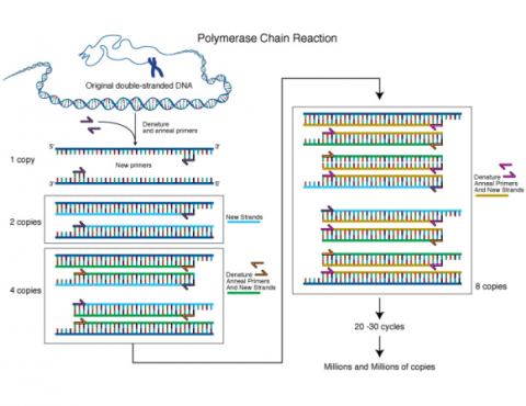
Various molecular methods have been developed to visualize SNPs or INDEL polymorphisms at low cost and high throughput, which will be presented in detail in the Molecular Genetics and Biotechnology course. The main use of those SNPs and INDEL polymorphisms is as molecular markers. By genetic mapping as described above, linkage between genes affecting agronomic traits or morphological characters, and DNA-based SNP or INDEL markers can be established. It can be more effective in the context of plant breeding, to select indirectly for such DNA markers, than directly for target genes. This is due to lower costs for DNA analyses, the ability to run multiple such assays (for multiple target genes) in parallel, the ability to select early and to discard undesirable genotypes or to perform selection before flowering, codominant inheritance of markers, among others.For example, both ginkgo trees (Ginkgo biloba) and asparagus (Asparagus officinalis) are dioecious species. Male plants are preferred for ginkgo tree because fruits produced from female trees have an unpleasant smell whereas male asparagus plants are preferred because of their higher yield potential. Unfortunately, sex expression will take years to occur for both species. If a DNA marker that either directly affects sex expression or is linked to genes that affect sex expression can be identified, selection of male plants can be conducted in early seedling stage rather than waiting for many years. Occurrence of environmental conditions favoring selection for disease, insect-resistant plants or drought-tolerant plants such as the prevalence of the particular disease or insect or drought is not always reliable. Selection using DNA markers can overcome these limitations as they are not affected by the environment.
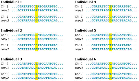
Polymorphism
Polymorphism involves one of two or more variants of a particular DNA sequence. The most common type of polymorphism involves variation at a single base pair, also called single nucleotide polymorphism (SNP) (Fig. 22). Polymorphisms can also be much larger in size and involve long stretches of DNA. Tandem repeat is a sequence of two or more DNA base pairs that is repeated in such a way that the repeats are generally associated with non-coding DNA. In contrast, SNPs can sometimes be identified that occur within coding sequences (that is within genes), as well as in non-coding DNA.
Types of Biochemical/Molecular Markers
There are a variety of biochemical and molecular markers available. Table 2 on the next page summarizes features of a number of the common ones:
- RFLP — Restriction Fragment Length Polymorphisms
- RAPD — Random Amplified Polymorphic DNA
- AFLP — Amplified Fragment Length Polymorphisms
- SSR — Simple Sequence Repeats (also known as microsatellites)
- SNP — Single Nucleotide Polymorphisms
- VNTR — Variable Number of Tandem Repeats
Widely-Used Markers
| Isozymes | RFLP | RAPD | AFLP | SSR | SNP | |
| Protein- or DNA-based |
Protein-based | DNA-based | DNA-based | DNA-based | DNA-based | DNA-based |
|---|---|---|---|---|---|---|
| No. of loci | 30-50 | 100s | ~Unlimited | ~Unlimited | 10s | 10s |
| Degree of polymorphism | Low-medium | Meduim-high | Medium-high | Medium-high | High | High |
| Nature of gene action | Codominant | Codominant | Dominant | Dominant | Codominant | Codominant |
| Reproducibility | High | High | Low-medium | Medium-high | High | High |
| Amount of DNA per sample | Not applicable | mg | ng | ng | ng | ng |
| Method* | Biochemical | DNA-DNA hybridization | PCR | PCR | PCR | PCR |
| Ease of array? | Easy | Difficult | Easy | Moderate | Easy-moderate | Easy |
| Can be automated? | Difficult | Difficult | Yes | Yes | Yes | Yes |
| Equipment cost | Inexpensive | Expensive | Moderate | Expensive | Expensive | Expensive |
| Development cost | Inexpensive | Expensive | Moderate | Expensive | Very | Expensive |
| Assay cost | Inexpensive | Expensive | Moderate | Expensive | expensive | Expensive |
* ‘PCR’ means Polymerase Chain Reaction amplification of genomic DNA fragments, a method that uses short, single-stranded DNA sequences, known as primers, to hybridize with the sample DNA Table 2. Comparison among widely used molecular markers. Adapted from Nageswara-Rao and Soneji, 2008.
SSR and SNP Markers
SSR markers remain useful to plant breeders due to their abundance and convenience with which they are assessed, but they serve most likely as linked markers. SNP markers, however can either be linked to or directly reside in a gene of interest and are hugely abundant. For these reasons, they are increasingly becoming the marker of choice.
Uses of Molecular Markers
Molecular markers are useful for both applied and basic genetic research. Here are some examples:
Indirect selection criteria in breeding programs (marker-assisted selection)
This is one of the most important and widely used molecular techniques in applied plant breeding programs today. RFLPs, SSRs, and SNPs enable breeders to indirectly select for a desired trait. Ordinarily, the DNA sequence of a molecular marker does not itself code the gene for the trait, but rather, its presence is correlated or linked with the gene for the particular trait. Thus, the breeder can indirectly select for the trait by directly selecting for the molecular marker—the DNA fragment and the gene encoding the trait are linked. The closer their physical proximity on a chromosome, the greater the probability that they will remain linked and not be separated through a recombination event in subsequent generations. As long as the gene for the trait and the marker remain linked, the marker is a useful selection criterion. Ultimately, however, potential lines still must be field-tested to verify the expression of the desired phenotype.
Identify quantitative trait loci (QTLs)
Molecular markers linked to genes contributing to the expression of polygenic or quantitative traits can be used to more efficiently identify and select individuals possessing the genes. It is more difficult to use conventional breeding approaches to identify plants that have accumulated the genes necessary to obtain the desired quantitative trait.
Genetic mapping
Molecular markers provide a means to map genes to more specific chromosome segments than is possible using visible markers.
Determine genetic relationships
The more molecular markers individuals have in common, the more closely related they are.
Genetic Diversity and Conservation
Genetic relationships within families, genera, species, or cultivars can be determined from molecular markers. Much information about the evolution of crops has been learned using molecular markers. The markers also enable breeders to monitor the genetic diversity among breeding lines to broaden the genetic base and reduce the risk of widespread genetic vulnerability to detrimental conditions.
Molecular Marker ‘Fingerprints’
Individuals possessing more markers in common than could occur by random chance are closely related. Such molecular fingerprints have been used successfully in court to prove the misappropriation of proprietary breeding lines.
Isolate genes
Molecular markers are used to map candidate genes on a much finer scale and can eventually isolate candidate genes by positional cloning. Isolated genes can be used to study gene regulation or to directly improve agronomic performance by genetic transformation. Although molecular markers have many applications and provide useful tools to plant breeders, lines must still be evaluated under normal production conditions before their release.
References
Falconer, D.S., and Trudy F.C. Mackay. Introduction to Quantitative Genetics (4th edition). San Francisco, CA: Benjamin Cummings.
Fehr, Walter R. 1987: Principles of Cultivar Development. Macmillan Publishing Company: New York.
Nageswara-Rao, M., J.R. Soneji, C. Chen, S. Huang, and F.G. Gmitter. 2008. Characterization of zygotic and nucellar seedlings from sour orange-like citrus rootstock candidates using RAPD and EST-SSR markers. Tree Genet Genomes. 4:113-124. DOI: 10.1007/s11295-007-0092-2
Neuffer M.G., Coe, E.H. and Wessler, S.R. (1997) Mutants of Maize. Plainview, NY: Cold Spring Harbor Laboratory Press
NIH-NHGRI (National Institutes of Health. National Human Genome Research Institute). 2011. Talking Glossary of Genetic Terms. [available online September 23, 2011, http://www.genome.gov/glossary/.
Neuffer M.G., Coe, E.H. and Wessler, S.R. (1997) Mutants of Maize. Plainview, NY: Cold Spring Harbor Laboratory Press
Pierce, Benjamin A. 2008: Genetics: A Conceptual Approach. W.H. Freeman and Company: 160-199, 335-339. New York, NY.
Rafalski, A. 2002 Applications of single nucleotide polymorphisms in crop genetics. Current Opinion in Plant Biology 2002, 5:94–100
Russell, Peter J. 2012: iGenetics: A Molecular Approach. Pearson Education, Inc., San Francisco, Calif.
How to cite this chapter: Lübberstedt, T., A. Campbell, D. Muenchrath, L. Merrick, S. Fei, and W. Suza. 2023. Linkage. In W. P. Suza, & K. R. Lamkey (Eds.), Crop Genetics. Iowa State University Digital Press. DOI: 10.31274/isudp.2023.130
definition
Polyploid with multiple chromosome sets derived from a single species.
A test of how much a given distribution deviates from the expected.
χ2=∑[(observed−expected)^2/expected]
