
Chapter 6: Optimization of Product Pipeline
Rita H. Mumm
Response to Selection, R
The cycle of cultivar improvement is implemented as a process of cultivar development, which is designed to produce a pipeline of improved cultivars that achieve the specific product target (Fig. 1).
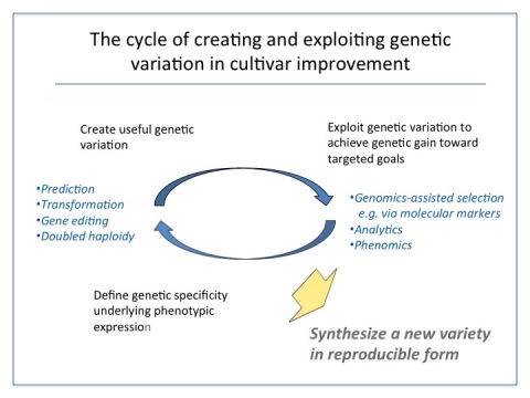
Generally speaking, top-performing individuals are selected from a base population with mean performance, µ, to serve as parents. Progeny produced from these parents are evaluated, with the best selected to serve as parents of the next cycle of selection.
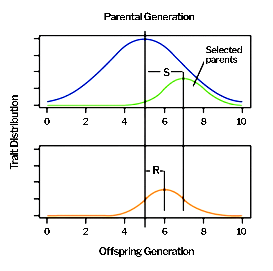
Narrow sense heritability ([latex]h^2[/latex]) is the portion of the genetic variance that can be transmitted to the next generation. It reflects the ratio of R to S:
[latex]\large h^{2} = \dfrac{R}{S}[/latex]
Factors Influencing R
The efficiency of the process can be measured in terms of R, which represents the response to selection.
[latex]\large R=h^{2}S[/latex]
We have seen in earlier chapters that R can also be expressed as:
[latex]\large R=ih^{2}σ_{\small P}[/latex]
[latex]\large R=i\bigg(\dfrac{σ^2_{\small A}}{σ^2_{\small P}}\bigg)σ_{\small P}[/latex]
[latex]\large R=\dfrac{i\;σ^2_{\small A}}{σ_{\small P}}[/latex]
[latex]\large R=ihσ_{\small A}[/latex]
where:
[latex]i[/latex] is selection intensity,
[latex]h^2 [/latex] is narrow sense heritability for the trait(s) under selection,
[latex]σ^2_{\small A}[/latex] is the additive genetic variance,
[latex]σ^2_{\small P}[/latex] is the phenotypic variance,
[latex]\small A[/latex] is additive genetic standard deviation,
[latex]\small P[/latex] is phenotypic standard deviation,
[latex]h[/latex] is the square root of [latex]h^2 [/latex] and refers to the accuracy of selection.
Furthermore, the rate of genetic gain (ΔG) over time can be expressed as:
[latex]\large \Delta G=\dfrac{R}{L}[/latex]
where [latex]L[/latex] is the length of a breeding cycle.
Which of the factors influencing R and ΔG are impacted by choices the breeder makes?
R as an Efficiency Indicator
Optimization of the product pipeline promotes maximal response to selection in the shortest amount of time at a comparative cost to produce improved cultivars that meet the needs of farmers and end-users.
Through process design, the breeder can affect the efficiency of the pipeline in developing improved cultivars. R is an efficiency criterion that can be used to compare various process design options to create a pipeline that maximizes ∆G over time.
Let’s take a look at how to utilize R as a measure of process efficiency…
More on Factors Influencing R
We have seen R expressed in a number of ways and these can be expanded further to elucidate more features of the breeding and testing regime over which the breeder has control.
For example:
[latex]\large R=h^{2}S[/latex]
where S is the selection differential, [latex]S = μ_S - μ[/latex]
[latex]\large R=\frac{σ^2_{\small A}}{σ^2_{\small P}}S[/latex]
[latex]\large R=\dfrac{σ^2_{\small A}}{σ^2_{\small P}}kσ_{\small P}[/latex] where [latex]k[/latex] is the number of phenotypic standard deviations between [latex]μ_S - μ[/latex]
[latex]\large R=\dfrac{k(c)(f)σ^2_{\small A}}{σ_{\small P}}[/latex]
where:
[latex]c[/latex] = parental control factor
[latex]f[/latex] = fraction of [latex]σ^2_{\small A}[/latex] among progeny being tested.
e.g., [latex]HS=\frac{1+F}{4}[/latex] where [latex]F[/latex] is the inbreeding coefficient of half sibs.
Impact of Parental Control
The parental control factor (c ) reflects the relationship between the entity used for identifying genotypes (selection unit) and the entity used to produce the next generation (recombination unit).
Note that:
- c = ½ when the selection unit is the same as the recombination unit and only female parents are selected
- c = 1 when the selection unit is the same as the recombination unit and both parents are selected
- c = 2 when the selection unit is not the same as the recombination unit; the recombination unit is the selfed seed or a clone of the selected.
For example, mass selection practiced with pollen control is twice as effective as without pollen control, all other factors being equal:
[latex]\Large R = \frac{k(1)(1)σ^2_{\small A}}{σ_{\small P}} \small { \text{(with pollen control)}} \large {\text { vs. }} \Large R = \frac{k(\frac{1}{2})(1)σ^2_{\small A}}{σ_{\small P}} \small {\text{ (without pollen control)}}[/latex]
It is easy to see that by conducting controlled pollinations using only selected lines, twice the genetic gain can be made in comparison to recombining female parents that have produced seed through uncontrolled pollination. This can be done when selections (for both male and female lines) are made prior to pollination.
Impact of the Form of the Selection Unit
In the expression of [latex]R[/latex], the variable [latex]f[/latex] has to do with the form of the selection unit. If half-sib progeny produced from the breeding crosses are subject to evaluation, then the proportion of the additive genetic variance represented is ¼. Likewise, if full-sib progeny are evaluated, then f = ½.
For example, full-sib selection is more effective than selection among half-sib progeny, all other factors being equal:
[latex]\Large R = \frac{k(1)(\frac{1}{2})σ^2_{\small A}}{σ_{\small P}}\small { \text{(full-sib selection)}}\large {\text { vs. }}\Large R = \frac{k(1)(\frac{1}{4})σ^2_{\small A}}{σ_{\small P}} \small { \text{(half-sib selection)}}[/latex]
Full-sibs account for twice the additive variance compared to half-sibs.
Furthermore, [latex]f[/latex] considers the level of inbreeding ([latex]F[/latex]) among the progeny. [latex]F[/latex] is assumed to be zero in the F2 generation; whereas, with fully homozygous progeny, [latex]F=1[/latex].
Assuming epistasis to be negligible, the genetic variability among families with or without inbreeding depends on the types of families under selection.
- Half-sib = [latex]\frac{1+F}{2}σ^2_{\small A}[/latex].
- Full-sib = [latex]\frac{1+F}{2}σ^2_{\small A} + \frac{(1+F)^2}{4}σ^2_{\small D}[/latex].
- Selfed = [latex](1+F)\,σ^2_{\small A} + \frac{1}{4}(1-F)(1+F)\,σ^2_{\small D}[/latex]; (Note that, with fully homozygous inbreds such as doubled haploid lines, this expression reduces to [latex]2σ^2_{\small A}[/latex]).
- Clones = [latex]σ^2_{\small A} + σ^2_{\small D}+σ^2_{\small I}[/latex].
The numerator of [latex]R[/latex] considers only the additive variance because only additive variation can be transmitted to progeny in a diploid species. However, other forms of genetic variation (e.g. dominance variance) contribute to the denominator of [latex]R[/latex] which we will explore later in this chapter.
The Impact of k on R
With [latex]k[/latex] denoting the number of phenotypic standard deviations that the mean of the selected differs from the base population mean, [latex]k[/latex] is the same as  (selection intensity; shown in earlier expressions of [latex]R[/latex]). Although individuals in the extremes of the distribution may be superior, they are rare. The chance of producing, identifying, and selecting individuals in the extremes of the distribution curve is enhanced as the number of lines tested increases. It is difficult to increase [latex]k[/latex] without concomitantly increasing the population size. Otherwise, the risk is depleting genetic diversity.
This relationship is illustrated in the following example: 10% selection from a population size of 10 means that 1 individual is selected; no genetic diversity remains for the next round of selection.
In contrast, 10% selection from a population size of 250 means that 25 individuals are selected. Additionally, a sufficient number of selected individuals to be recombined for the next cycle of selection contributes to reducing the potential effects of genetic drift.
In fact,[latex]k[/latex] is related to [latex]p[/latex], the proportion of selected individuals in the base population. Falconer (1989; Appendix Table A) shows the relationship between [latex]i[/latex] (i.e. [latex]k[/latex]) and [latex]p[/latex] and [latex]x[/latex], the latter being the difference between the threshold point of selection (i.e. truncation point) and the base population mean, expressed in standard units.
Plant breeders often set [latex]p[/latex] at certain values; [latex]p[/latex] translates to values of [latex]x[/latex] in the Z Table. Note that [latex]x[/latex] for 5% and for 1% are the familiar statistics from the Z Table, 1.645 and 2.326, respectively (Table 1).
| [latex]p[/latex] (%) | [latex]x[/latex] | [latex]i[/latex] (i.e. [latex]k[/latex]) |
|---|---|---|
| 0.1 | 3.090 | 3.367 |
| 0.5 | 2.576 | 2.892 |
| 1 | 2.326 | 2.665 |
| 2 | 2.054 | 2.421 |
| 5 | 1.645 | 2.063 |
| 7.5 | 1.440 | 1.887 |
| 10 | 1.282 | 1.755 |
| 25 | 0.674 | 1.271 |
| 50 | 0 | 0.798 |
Other Ways to Maximize R
So far we have looked at ways to maximize [latex]R[/latex] by enlarging the numerator in the [latex]R[/latex] equation:
[latex]\large R=\dfrac{k(c)(f)\,\sigma _{A}^{2}}{\sigma _{P}}[/latex]
In addition, [latex]R[/latex] can be optimized by reducing the denominator.
Partitioning Phenotypic Variation
We know that phenotypic variation is a function of variation attributable to genotype, environment, genotype-by-environment interaction (GxE ), and error.
Simply put, the denominator can be expressed as:
[latex]\large \sigma_{\small {P}}=\sqrt{\frac{\sigma ^{2}}{rt}+\frac{\sigma^2_{GE}}{t}+\sigma^{2} _{G}}[/latex]
where:
[latex]σ^2[/latex] is experimental error
[latex]\sigma^2_{\small GE}[/latex] is variance due to genotype by environment interaction
[latex]\sigma^2_{\small G}[/latex] is genetic variance
[latex]r[/latex] is the number of replications in testing
[latex]t[/latex] is the number of environments (which could include locations, seasons, years, cultural practices, etc.).
Accordingly, this expression can be expanded, with [latex]\sigma^2_{\small P}[/latex] expressed as:
[latex]\large \sigma _{p}=\sqrt{\frac{\sigma_{w}^{2} }{nrly}+\frac{\sigma_{e}^{2} }{rly}+\frac{\sigma_{GLY}^{2} }{ly}+\frac{\sigma_{GY}^{2} }{y}+\frac{\sigma_{GL}^{2} }{l}+\sigma _{G}^{2}}[/latex]
where:
[latex]\sigma_{w}^{2}[/latex] is the within-plot experimental error variance,
[latex]\sigma_{e}^{2}[/latex] is the variance among replications,
[latex]\sigma_{GLY}^{2}[/latex] is variance due to genotype by location by year interaction,
[latex]\sigma_{GY}^{2}[/latex] is variance due to genotype by year interaction,
[latex]\sigma_{GL}^{2}[/latex] is variance due to genotype by location interaction,
[latex]\sigma_{G}^{2}[/latex] is genetic variance,  is the number of plants per plot,
[latex]r[/latex] is the number of replications in testing,
[latex]l[/latex] is the number of testing locations
[latex]y[/latex] is the number of years of testing.
Note that the mean square error in ANOVA is comprised of within-plot and among-plot variation:
[latex]\large \frac{\sigma ^{2}}{rt}=\frac{\sigma _{w}^{2}}{nrly}+\frac{\sigma _{e}^{2}}{rly}[/latex]
Moreover, the within-plot experimental error variance [latex]\sigma _{w}^{2}[/latex] can be partitioned further into variation due to environmental effects ([latex]\sigma _{u}^{2}[/latex]) and variation due to genetic differences among plants ([latex]\sigma _{wg}^{2}[/latex] ):
[latex]\large \sigma _{w}^{2}=\sigma _{u}^{2}+\sigma _{wg}^{2}[/latex]
Environmental effects [latex]\sigma _{u}^{2}[/latex] include micro-scale effects within the plot that would cause genetically identical plants to perform differently (e.g. soil fertility, soil type, soil moisture, shading). Within-plot genetic variation [latex]\sigma _{wg}^{2}[/latex] is attributable to segregation such as might occur before lines are fully inbred.
In addition, variation attributable to GxE can be expanded. Thus,
[latex]\large \frac{\sigma_{GE}^{2}}{t}=\frac{\sigma _{GLY}^{2}}{ly}+\frac{\sigma _{GY}^{2}}{y}+\frac{\sigma _{GL}^{2}}{l}[/latex]
The variation attributable to GxE could be expanded further if needed to include variance due to ‘seasons’ or cultural practices (e.g. irrigation vs. dryland).
Maximizing R Through Trial Design
 can be maximized through design of evaluation trials. Uniform fields will contribute to less variation within plots and among replications, thus smaller [latex]\sigma^2_w[/latex] and [latex]\sigma^2_e[/latex], respectively.
To maximize [latex]R[/latex], [latex]\sigma_{\small{P}}[/latex] can be reduced by increasing the number of reps ([latex]r[/latex]), number of locations ([latex]l[/latex]), and/or number of years ([latex]y[/latex]) in evaluation for selection. Relatively speaking, increasing locations or years in testing has a greater effect than increasing replications (that is, [latex]l[/latex] and [latex]y[/latex] have the opportunity to reduce more components of variation since they are featured in the denominators more often than [latex]r[/latex]).
[latex]R[/latex]will increase as the number of plants per plot ([latex]n[/latex]) is increased. When there is only 1 plant per plot, [latex]n=1[/latex]. In family selection, the value of [latex]n[/latex] is determined by the number of plants in the plot. For example, with F3 family selection involving 30 plants per plot, [latex]n=30[/latex]. The effect of increasing plant numbers per plot as it relates to [latex]\frac{\sqrt{\sigma^2_{w}}}{n}[/latex] can be seen in the following table (Table 2).
Furthermore, error variance components, [latex]\sigma^2_w[/latex] and [latex]\sigma^2_e[/latex], can be reduced by controlling human error such as mistakes in recording the evaluation data.
| [latex]n[/latex] | [latex]\frac{\sqrt{\sigma^2_{w}}}{n}[/latex] |
|---|---|
| 1 | 22.3 |
| 2 | 15.8 |
| 3 | 12.9 |
| 4 | 11.2 |
| 5 | 10.0 |
| 10 | 7.1 |
| 20 | 5.0 |
| 30 | 4.1 |
| 60 | 2.9 |
| 90 | 2.4 |
The Impact of GxE on R
The impact of GxE can be reduced by evaluating progeny in multiple locations and over multiple years. Variation due to GxE is captured in [latex]\sigma_{\small {GLY}}^2[/latex] (variance due to genotype by location by year interaction), and [latex]\sigma_{\small {GY}}^2[/latex] (variance due to genotype by year interaction), and [latex]\sigma_{\small {GL}}^2[/latex] (variance due to genotype by location interaction). Because GxE interferes with the ranking of the progeny and identification of top performers, it has serious ramifications for accuracy in selection.
For crops in which GxE features largely, the greatest genetic gain per year is realized by maximizing  at the expense of [latex]r[/latex] (i.e. 1-rep trials at the greatest number of locations possible). The trade-off here is cost, since with a fixed number of reps, it is more expensive to include more locations than to have multiple reps at fewer locations. (More on choice of locations later in this chapter.)
Note that [latex]\sigma_{\small {GY}}^2[/latex] and [latex]\sigma_{\small {GLY}}^2[/latex] cannot be measured or effectively reduced without testing over multiple years. Obviously, the trade-off is time. As an alternative option, additional locations may be substituted for added years.
Choosing Testing Environments to Maximize R
Choice of testing sites is critical to the selection decisions that will be made in the process of cultivar development. Selections will be made based on phenotypic performance at these sites for traits pertinent to the product target.
Prospective testing sites are assumed to represent a sample of environments from the target market region. However, realistically there may be hundreds of thousands of “environments” within the target region, considering the many factors that play a role in determining the environment (e.g. geography, altitude, season, maturity zone, soil types, topography, farmer production management system including tillage, fertilization, mechanization, and water regime, etc.). Selection in cultivar development is aimed at the identification of genotypes that have high mean value in the target set of environments.
The usefulness of a testing site can be characterized in terms of:
- Ability to differentiate between genotypes
- Accuracy of selection: [latex]h[/latex]
- Correlation of test environment with target environment within the market region.
The purpose of testing in cultivar development is to reveal genetic differences among test entries and the magnitude of those differences, and to indicate whether performance of any is sufficient to meet the stated product target. Trial design and implementation have an important role in this. However, some types of environments (e.g. drought stress and other abiotic stress environments) inherently have greater variability due to non-genetic factors.
Heritability ([latex]h^2[/latex]) can be considered a measure of the signal-to-noise ratio in estimating breeding value; GxE interaction and experimental error reduce the effectiveness of selection:
[latex]\Large h^{2}=\frac{\sigma _{A}^{2}}{\frac{\sigma ^{2}}{rt}+\frac{\sigma_{\small{GE}}^{2}}{t}+\sigma _{\small{G}}^{2}}[/latex]
Accuracy of selection or [latex]h[/latex] is defined as the correlation between breeding value and phenotypic value and can be computed as the square root of narrow-sense heritability ([latex]\sqrt{ h^2}[/latex]) (Falconer 1989); it is considered a measure of repeatability. Therefore, the accuracy of selection decisions depends on reducing GxE and experimental error in testing. Accuracy of selection often differs across testing sites, but this statistic alone is not sufficient to establish the value of a testing environment.
Because selections are based on a sample of the entire population of environments, selection will be truly accurate only if the observed phenotype in that particular environment or set of environments is highly correlated with mean performance in the target environment.
Allen et al. (1978) suggested that an appropriate measure of the usefulness of a test environment is [latex]r\sqrt{ h^2}[/latex] where [latex]r[/latex] is the genetic correlation of performance in the test environment with performance in the target environment.
Challenges in Choosing Testing Environments
Ideally, test environments are discriminating among genotypes as well as representative of the target market region.
Some questions to consider in identifying useful test sites are:
- Are there multiple target environments (i.e. mega-environments) within the target market region?
- Within a specific mega-environment, what are the most representative and discriminating test sites?
- How many test sites (and replications within a trial) can be implemented each year on my budget?
With a defined budget, it is important to understand meaningful mega-environments within the market region and to utilize testing environments that provide the most useful information in identifying “best” genotypes.
GxE Interaction Patterns
Ideally, an improved cultivar with wide adaptation across the entire defined target market is developed. This is relatively easy if GxE is negligible across the market region. In this case, test entries would perform similarly across test sites; differences between entries would not change from one environment to the next, and thus rankings would not change.
Sometimes the level of GxE is such that differences between lines change in magnitude from one environment to the next, yet rankings of entries based on performance still hold.
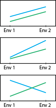
Crossover interaction is evident when differences between entries change substantially, resulting in rankings being flipped. A top entry at one location may be the worst-performing entry at another (Fig. 2).
- Parallel pattern: no interaction.
- Non-parallel but rankings still hold.
- Crossover interaction: Rankings are flipped!
With consistent patterns of GxE over years, there are groups of locations that consistently share the best set of genotypes or cultivars, and this implies a repeatable pattern that can be used to exploit GxE in cultivar development. Strategically, it means that selection will focus on specifically adapted genotypes for each mega-environment. Thus, each mega-environment becomes a “target environment” and test sites within that mega-environment must be representative of that target environment.
Tools to Aid in Evaluating Testing Environments
There are a number of tools that can aid in answering the questions posed (see slide entitled Challenges in Choosing Testing Environments in this chapter).
Cluster analysis has been used to identify similar types of environments and categories of environments. In addition, the performance of test entries grown at one location can be correlated with the performance of the same set of entries at other locations and performance overall.
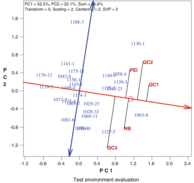
AMMI (Additive Main Effects and Multiplicative Interaction) analysis has been used to dissect GxE via principal components analysis and characterize yield stability over environments (Gauch 1992). A biplot can be produced to graphically display the relationships of environments with each other and with test entries.
GGE biplot involves only genotype and GxE interaction effects in the principal components analysis. A biplot displaying environments and entries based on the first two principal components, PCA1 and PCA2, provide insights into the number of mega-environments represented in the data and indicates test environments that are most representative and discriminating. Graphics can be unscaled or scaled in different ways (e.g. by the standard deviation of an entry mean within environment or the standard error within environments).
In particular, when GGE biplots are scaled according to the heritability of the trait measured, the length of the vector extending from the origin to the environment is proportional to the square root of heritability ([latex]r\sqrt{h^2}[/latex]) in the environment. This type of analysis is referred to as a heritability-adjusted GGE biplot (Yan and Holland 2010) (Fig. 3). The angles between environment vectors approximate the genotypic correlation between environments.
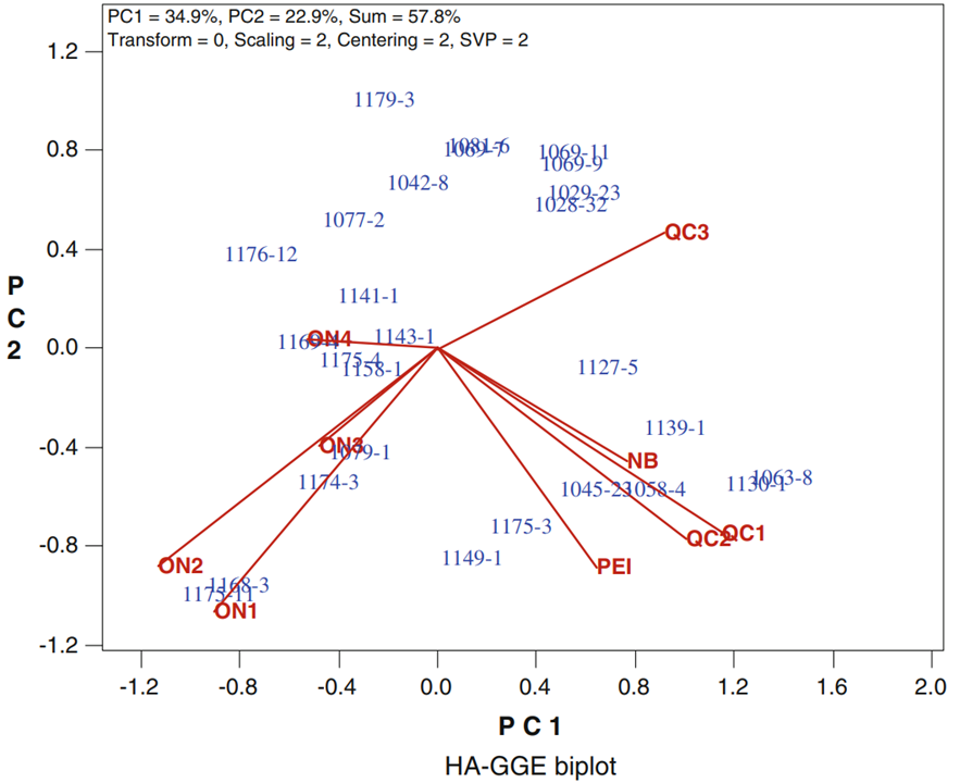
Furthermore, this type of analysis provides approximations of [latex]r\sqrt{h^2}[/latex] for each test environment, which is proportional to the predicted [latex]R[/latex] in the mega-environment based on the data from the test environment. Thus, it delivers information the breeder can use in choosing environments that maximize [latex]R[/latex] in a way that fits within budgetary constraints.
Impact of Type of Gene Action on R
In the expression of [latex]R[/latex], the denominator includes all the genetic variance while only the additive genetic variance is included in the numerator (since only additive genetic variance can be transmitted to progeny):
[latex]\large R=\large\frac{k(c)(f)\sigma^{2} _{A}}{\large \sqrt{\frac{\sigma^{2} _{w}}{nrly}+\frac{\sigma^{2} _{e}}{rly}+\frac{\sigma^{2}_{GLY}}{ly}+\frac{\sigma^{2}_{GY}}{y}+\frac{\sigma^{2}_{GL}}{l}+\sigma^{2}_G}}[/latex]
The genetic variation accounted for in the denominator will depend in part on the gene action of the trait being improved. This means that traits that are substantially influenced by dominant or epistatic gene action are generally less responsive to phenotypic selection. And generally, such traits are characterized by lower heritability. Typically, epistasis is assumed to be negligible in estimating [latex]R[/latex].
In addition, the family structure of the population under improvement will impact [latex]R[/latex]. As shown above, the genetic variability among families with or without inbreeding depends on the types of families under selection. For example, half-sib families reflect additive genetic variance only, whereas full-sib families reflect both additive and dominance genetic variance. In estimating [latex]R[/latex] using half-sib families, only additive genetic variance would be included in the denominator.
See Fehr, 1991, Chapter 17 for examples of comparing alternative breeding methods for predicted gain ([latex]R[/latex]).
Breeders cannot change gene action. However, there are ways to deal with low heritable traits, including the use of indirect selection through secondary traits that may offer higher selection efficiency.
Use of Indirect Selection to Increase R
This really relates to the type of screen that is utilized to select for a given trait in the product target. Generally speaking, the screen should be accurate and relevant to field performance. As discussed in Chapter 2, to improve Character X, selection may be based on another Character Y. Indirect selection will result in a relatively greater genetic gain for Character X than directly selecting for it if:
[latex]\large r_{\small G_{XY}} h_{\small Y} > h_{\small X}[/latex]
where:
[latex]r_{\small G_{XY}}[/latex] is the genetic correlation between Characters X and Y,
[latex]h_{\small X}[/latex] and [latex]h_{\small Y}[/latex] represent the square root of the narrow sense heritability for Characters X and Y, respectively.
Marker-assisted selection (MAS) is one type of indirect selection. Selection for superior individuals is based on the genotype of specific marker(s) instead of phenotype (or in addition to phenotype). Since marker genotypes are completely heritable (thus,  is 1), the efficiency of marker-based selection is a function of the heritability of the primary trait and the proportion of additive genetic variance of the primary trait attributable to the markers.
When the proportion of additive genetic variance accounted for by the markers is greater than the heritability of the primary trait, then [latex]r_{\small G_{XY}}[/latex] is greater than [latex]h_{\small X}[/latex], and MAS holds an advantage.
Impact of L on ∆G
Response to selection over time is given by the equation for the rate of genetic gain:
[latex]\large \Delta G=\dfrac{R}{L}[/latex]
Obviously, the length of the breeding cycle , L, is a significant element in maximizing G .
What are ways in which L can be reduced?
- By increasing the number of generations advanced per year in breeding to homozygosity. This may involve use of growth chambers, greenhouses, off-season nurseries, and continuous nurseries that facilitate more than one generation per year and may involve breeding methods like single-seed descent.
- Use of trait screens that facilitate selection before pollination (so that both parents are from the selected group) or even facilitate selection before planting (marker-based selection using plant seed tissue for DNA extraction).
- Reducing the length of the time required for the testing regime. This may involve a trade-off between the number of years of testing and the number of locations grown each year in order to maintain a comparable [latex]R[/latex].
These ways are but some of the many ways that [latex]L[/latex] can be reduced.
Can you think of others?
Check out this YouTube video that shows approaches to speed breeding devised by the Hickey Lab at the University of Queensland.
Accelerating Development Time
Just as development time can be reduced by shortening the length of a generation, still another way to realize efficiency is in terms of time to develop an improved cultivar that reflects a specific magnitude of genetic gain. After all, we are interested in releasing improved cultivars to farmers in the shortest amount of time required, depicted in the equation below.
[latex]\large Time = R * L[/latex]
Development time required involves a trade-off between the magnitude of [latex]R[/latex] per cycle ([latex]L[/latex]) and the number of cycles of selection. If greater gain can be achieved per cycle, fewer cycles (and less time) may be needed to achieve a particular genetic gain.
Having discussed factors to increase [latex]R[/latex], one that is recognized for reducing time to market is population size. With enough increase in population size, the gain achievable in two cycles of selection could potentially be realized in one.
Recap
Study of the formulas for [latex]R[/latex] has revealed several ways for increasing response to selection:
- Select a smaller proportion of individuals; coordinate higher selection intensity with increased population size to avoid loss of genetic diversity and potential effects of genetic drift.
- Utilize breeding methods that allow for control of both parents; choice of pollen parent as well as seed parent to produce progeny for the next cycle of selection offers great advantage. Furthermore, utilizing approaches to allow recombination of selfed seed or clones of selected individuals (vs. remnant seed) adds to greater progress.
- Increase the coefficient of [latex]σ^2_{\small A}[/latex]; [latex]f[/latex] can be increased through the choice of selection unit (e.g., full-sib families vs. half-sib families) and by evaluating more highly inbred materials (e.g. recombinant inbred lines vs. early generation segregating lines).
- Deploy appropriate experimental designs in testing to minimize environmental variation and error. For advanced yield trials involving high numbers of entries, incomplete block designs can be used to further partition blocks in the field into more homogeneous units. Include multiple locations and multiple years to partition and account for variation due to GxE. Increase replications to the greatest extent feasible.
- Control within-plot variation through appropriate plot size (i.e. number of plants per plot). Conduct single-plant evaluations only with highly heritable traits.
- For lowly-heritable traits, consider the use of secondary traits as a basis for selection. Molecular markers may be useful if the markers aid in accounting for a greater portion of the additive genetic variance than phenotypic selection alone.
- Reduce the length of the cycle by shortening the time required for the breeding and testing of progeny.
- Reduce the number of cycles needed to achieve a particular magnitude of gain by increasing selection intensity through increased population size.
Thus, the breeder exerts tremendous influence on the response to selection and the rate of gain, simply through the choice of breeding strategies, methods, materials for testing, and the conduct of evaluations. Therefore, the design of the product pipeline which incorporates these features in the breeding and testing regime is critical to developing and releasing improved cultivars that meet farmer and end-user needs.
The breeder can utilize the formulas for [latex]R[/latex] to compare various options in the product pipeline for the greatest efficiency.
Improving Breeding Efficiency Through the Use of Technology
The term “technology” refers loosely to industrial science. That is, any applied science in the form of tools, machines, or methodologies used to solve real-world problems. In crop improvement, technology includes DNA-based approaches to selection as well as the tools and methods to accomplish the selection, machines such as drones to record data more efficiently, and processes such as doubled haploidy that are enabled through scientific application.
Two technologies are highlighted here as examples, considering their potential role in the product pipeline and ways to maximize the benefit of the technological investment:
- molecular markers, specifically applied to facilitate indirect selection
- doubled haploidy to accelerate development of homozygous lines from a breeding cross.
Boosting Breeding Efficiency Through Marker-Assisted Selection

Molecular markers can be used to select for individuals with favorable alleles at loci controlling traits of interest in close proximity to marker loci. Selection based on molecular marker genotype may contribute to breeding efficiency.
In potato, for example, Marker-Assisted Selection (MAS) can be used to address some of the critical challenges in cultivar development. Potato is a highly heterozygous, tetraploid crop with very complex product targets involving as many as 40 characteristics including disease and pest resistances, tuber appearance, quality, nutrient content, and stress tolerances, in addition to agronomic traits of yield, yield stability, and maturity (see Chapter 4). Evaluation is costly and time consuming. The process of New Line Development and New Line Evaluation can take 10+ years. Furthermore, many traits are highly influenced by the particular growing environment or correlated with conditions such as seed tuber size.
Many of the key traits are qualitative, controlled by a few genes, or are quantitative in nature but highly influenced by major genes. Yet, because potato is an autotetraploid, five distinct genotypes may be observed at any given locus (AAAA, AAAa, AAaa, Aaaa, aaaa) making progeny testing difficult.
Ideal Markers
There are various types of molecular markers, with Single Nucleotide Polymorphisms (SNPs) being the most widely used type today.
Ideally, the markers are:
- Co-dominant, revealing the detail of allelic composition
- “Perfect” (i.e. located within the gene itself, to avoid the chance of recombination between the marker and the tagged gene)
- Consistently reproducible (i.e. the assay results are consistent for each genotype, even across different laboratories)
- High-throughput (HTP) (i.e. amenable to automation for fast delivery of results and widespread application)
- Cost effective.
In potato, many single-gene traits have been mapped in addition to major genes contributing to the expression of quantitative traits.
Potential Advantages to Exploit with MAS
MAS may offer some significant advantages over phenotypic selection.
For example:
- Easier screening (e.g. resistance screening for potato cyst nematode)
- Screening at an earlier plant development stage
- Greater accuracy by eliminating classification errors due to environmental effects
- Selection can be applied outside of the market region and growing season (e.g. in an off-season nursery or greenhouse)
- HTP operation facilitates larger population sizes and higher selection intensity
- Fewer years of testing
- May be less expensive than phenotypic evaluation
Potential cost savings are just as important in optimizing the product pipeline as time savings, and depending on the situation at hand, may be more important.
Slater et al. (2013) compared the cost of applying MAS to screen for disease resistance in the second field generation (G2) against the cost of phenotypic evaluation of G2 selections. The MAS option was 37.3% of the cost of the phenotypic selection option. This strategy also provides the option to select for other markers associated with single-gene traits or major genes among G2 clones, with multiplexing marker assays as means to further the cost savings. In addition to cost savings, the MAS option resulted in a one-year time savings in cultivar development.
See Slater et al. 2013 for more detail.
Extracting the Most Value From Deployment of MAS
Often, the advantages provided through technology can be amplified further by tailoring the product pipeline for optimal fit or combining technologies.
Slater et al. (2014) exploited the advantages of MAS further in potato by combining MAS with selection based on estimated breeding value (EBV). By evaluating G2 clones for EBV, those individuals with high scores that may not possess the disease resistance sought through MAS are not discarded but recycled to increase the frequency of favorable alleles for other target traits. Those individuals selected by MAS and EBV are advanced to regional trials, reducing testing by two years. This enhances the time savings achieved overall to three years.
Although Slater et al. (2014) utilized pedigree information to compute EBVs, this could also be done through the use of markers using an approach like genomic selection.
See Slater et al. 2014 for more detail.
Boosting Breeding Efficiency Through Doubled Haploidy
With many crops, once a cross has been made to develop a breeding population, a major time lag occurs between F2 and the development of a fully inbred line. This time lag can be mitigated through early testing, yet we have seen that phenotypic measurement is most accurate and precise when non-segregating materials are used.
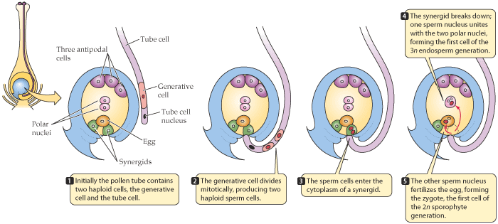
Doubled haploidy is a technology that can be used to by-pass the process of inbreeding, providing a quick route to homozygosity with a high degree of fidelity. With doubled haploid (DH) production systems available for more than 250 plant species, this technology manipulates the double fertilization process which gives rise to seed with a 2N embryo and a 3N endosperm (Fig. 6).
In maize, the use of an in vivo maternal haploid system via gynogenesis has become common. First reported by Stadler and Randolph in 1929, the system involves the use of an “inducer line” and typically also features a color marker system to facilitate the identification and confirmation of haploid individuals.
In vivo Maternal DH Production Process
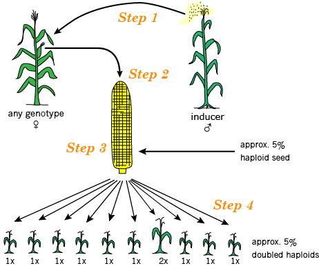
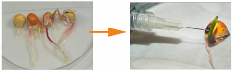
The basic steps involved in in vivo maternal DH production in maize are (Fig. 7):
- Pollinate donor plants (F1 or F2 progeny from a breeding cross) with inducer line
- Identify and recover haploid seed via color marker phenotype
- Germinate haploid seed and apply chromosome doubling agent
- Grow DHs to maturity & self-pollinate
Haploid Selection
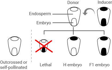
Much of the seed produced by pollinating the donor plants with the inducer line will be F1s, which are useless. A small proportion will be haploids which contain only genetic material from the donor line (the haploid induction rate is determined by the inducer line). And a fraction will be lethal mutants. There also may be some seed resulting from self-pollination or outcrossing since pollinations are made manually.
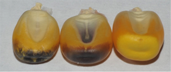
The color marker system makes it possible to sort the various types of seed. Since the color indicates genetic contribution from the donor, the haploid seed will show color only in the endosperm, not the scutellum which harbors the embryo (Fig. 8).
In real life, expression of the color markings is influenced by the genetic background (Fig. 9).
Chromosome Doubling Treatment
Once haploid seeds are recovered, these are germinated and then exposed to a chromosome-doubling agent to duplicate the chromosome content.
Recovering Doubled Haploid Lines
Those haploid plants that successfully doubled chromosome content are self-pollinated and grown to physiological maturity. The harvested selfed seed represents the new doubled haploid line. All seed on the ear is genetically identical and completely homozygous.
For more details on the in vivo maternal doubled haploid process in maize, see the YouTube clip from CIMMYT: “Doubled Haploids: A simple method to improve the efficiency of maize breeding.”
Extracting the Maximal Value from Deployment of Doubled Haploidy
Doubled haploidy offers the benefit of reduced cycle time. Plus, testing homozygous lines results in more precise estimates of performance than segregating lines, and thus affords more accuracy in selection decisions. Used to estimate QTL effects, DH lines again win over segregating lines.
Some organizations offer DH services so this step in the breeding process may be outsourced if desired. Nonetheless, there is an investment in tapping into this resource which can improve efficiency in cultivar development.
The big question is how to extract maximal value from the deployment of this technology. We will focus on three ways:
- The type of donor population
- Pre-selection of lines for haploid induction, sometimes referred to as “F2 enrichment”
- The structure of performance testing given the vast number of DHs that can be produced from a single breeding cross.
Best Population Type to Serve as Donor
Some options for the type of donor population to use to initiate doubled haploidy include F1, F2, and BC1. These population types differ regarding the number of meiosis, that is, the number of times cell division has taken place to produce reproductive cells. With meiosis comes recombination, and after all, it is new combinations of favorable alleles that we seek in developing improved cultivars!
Genetic theory tells us that the number of crossover events is less among DH lines compared to RILs. The evidence supporting this includes:
- Smith et al. (2008) found a mean of 15 recombinations per RIL versus 10 recombinations per DH genome developed from F1 donors
- Smith et al. (2008) found that the percentage of lines with ≥4 intact parental chromosomes (10 chromosomes in maize) was 37% among DHs and 13% among RILs.
DH lines developed from F2 donors allow for one more meiosis to occur. Work by Bernardo (2009) showed that DH F2 lines were no more than 3% lower in selection response than RILs and were up to 6% higher in selection response than DH F1 lines. Likewise, BC1 donors would offer the same advantage as F2 donors (compared to F1).
Although one more generation is required to produce the F2 or BC1 donors (compared to the F1 donors), it does not necessarily mean another year is required in development time. Off-season nurseries or greenhouses could be utilized to advance some/all generations and facilitate more generations per year. So this is a good trade-off!
Pre-Selection of Lines for Haploid Induction
Using F2 (or BC1) lines provides an opportunity for some selection to be performed before pollination with the inducer line. The rationale for such selection is to focus DH resources on individuals with greater genetic promise. Better donors should translate to greater genetic gain toward the product target.
Selection among F2 families based on single-plant performance could focus on high-heritability traits or marker genotype. Examples include:
- Plant morphology
- Disease resistance
- Favorable marker genotype for linked trait
- Against negative marker genotype for linked trait
- Increased or decreased frequency of recombinants in which repulsion linkages have been broken or favorable complexes of gene combinations have been preserved (Smith et al., 2008).
In a more elaborate scheme, Bernardo et al. (2010) proposed three cycles of genomic selection in a recurrent selection scheme as a means to enrich the frequency of favorable alleles for yield and other quantitative traits of interest.
The advantage of pre-selection of lines is to focus breeding and testing resources on lines with the greatest genetic potential, which should in turn result in the greatest genetic gain and higher [latex]R[/latex].
Performance Testing and Selection of DH Lines
With doubled haploidy, it is easy to produce a large number of progeny per breeding cross. And this can be accomplished in an accelerated timeframe (compared to inbreeding).
Through doubled haploidy, the breeder’s problem of having to wait until RILs are developed is solved. Now the issue is how to test the vast number of quickly-available inbred lines! An example of how to address this issue is briefly described below.
Assuming similar budgets Melchinger et al (2005), compared the rate of genetic gain ([latex]G[/latex]) achieved with a four-location preliminary yield test with a population of 250 segregating testcross progeny in maize with two-stage testing involving 739 DH lines at one location, followed by testing of 29 selections (from Year 1) at nine locations in a second season. The two-stage testing resulted in a nearly 20% increase in [latex]G[/latex] with the same resource investment.
Although the number of yield plots is the same in both cases, two-stage testing accommodates more lines and focuses a higher degree of scrutiny on the top performers. Thus, two-stage preliminary testing may be more effective in maximizing [latex]R[/latex] when doubled haploid technology is utilized to develop progeny.
To optimize the product pipeline and deliver improved cultivars to farmers most effectively and efficiently, consider each aspect of process design in breeding and testing as it relates to the factors influencing response to selection [latex]R[/latex] and rate of genetic gain ([latex]G[/latex]).
Technologies can be useful in boosting efficiency. The merit of applying any new technology can be judged in terms of its ability to increase genetic gain and the cost/benefit ratio. Once a decision is made to incorporate a new technology into the product pipeline, its value can be maximized by fine-tuning the pipeline process to take advantage of opportunities the technology affords to increase [latex]R[/latex] and reduce development time.
Finally, integration of all the components of the process is critical to a robust product pipeline that consistently produces improved cultivars. A chain is only as strong as its weakest link!
References
Allen, F.L., R.E. Comstock, and D.C. Rasmusson. 1978. Optimal environments for yield testing. Crop Sci. 18: 747-751.
Bernardo, R. 2009. Should maize doubled haploids be induced among F1 or F2 plants? Theor. Appl. Genet. 119:255-262.
Bernardo, R. 2010. Breeding for Quantitative Traits in Plants. 2nd edition. Stemma Press, Woodbury, MN.
Bernardo, R., R.E. Lorenzana, and P.J. Mayor. 2010. Exploiting both doubled haploids and cheap and abundant molecular markers in corn breeding. pp 40-53. In Proc. 46th Annual Corn Breeders’ School, 2010.
Falconer, D.S. 1989. Introduction to Quantitative Genetics, 3rd ed. John Wiley & Sons, New York, NY.
Fehr, W.R. 1991. Principles of Cultivar Improvement v1: Theory and Technique. Macmillan Publishing Company.
Gauch, H.G. 1992. Statistical Analysis of Regional Yield Trials: AMMI Analysis of Factorial Designs. Elsevier, Amsterdam, The Netherlands.
Geiger, H.H. 2009. Doubled haploids. pp641-657. In J.L. Bennetzen and S. Hake (eds), Handbook of Maize: Genetics and Genomics. Springer, New York, NY. https://doi.org/10.1007/978-0-387-77863-1_32
Melchinger, A.E., C. F. Longin, H.F. Utz, J.C. Reif. 2005. Hybrid maize breeding with doubled haploid lines: quantitative genetic and selection theory for optimum allocation of resources. Pp 8-21. In Proc. 41th Annual Corn Breeders’ School, March 2005.
Mumm, R.H. 2013. A look at seed product development with genetically modified crops: Examples from maize. J. Agricultural and Food Chemistry 61(35): 8254-8259. DOI 10.1021/jf400685y
Randolph, L.F. 1932. Some effects of high temperature on polyploidy and other variations in maize. Genetics 18: 222-229.
Slater, A.T., N.O.I. Cogan, J.W. Forster. 2013. Cost analysis of the application of marker-assisted selection in potato breeding. Molecular Breeding 32: 299-310. DOI 10.1007/s11032-013-9871-7
Slater, A.T., N.O.I. Cogan, B.J. Hayes, L. Schultz, M.F.B. Dale, G.J. Bryan, J.W Forster. 2014. Improving breeding efficiency in potato using molecular and quantitative genetics. Theor. Appl. Genet. 127: 2279-2292. DOI 10.1007/s00122-014-2386-8
Smith, J.S.C., T. Hussain, E.S, Jones, G. Graham, D. Podlich, S. Wall, M. Williams. 2008. Use of doubled haploids in maize breeding: Implications for intellectual property protection and genetic diversity in hybrid crops. Molecular Breeding 22: 51. https://doi.org/10.1007/s11032-007-9155-1
Yan, W., J.B. Holland. 2010. A heritability-adjusted GGE biplot for test environment evaluation. Euphytica 171: 355-369. DOI 10.1007/s10681-009-0030-5
How to cite this chapter: Mumm, R.H. (2023). Optimization of Product Pipeline. In W. P. Suza, & K. R. Lamkey (Eds.), Cultivar Development. Iowa State University Digital Press.
(1) A mega-environment is a group of locations that consistently share the best set of genotypes or cultivars across years (Yan and Rajcan, 2002).
(2) Categories of environments within the target market region that consistently share the best set of genotypes or cultivars across years.
Nurseries that facilitate planting and cultivation of materials at times other than the growing season in the target market region. For example, programs in temperate regions may seek facilities in the alternative hemisphere where seasons are flipped.
Continuous nurseries are located in geographic regions that permit the continual planting and cultivation of materials all year around. For example, tropical location sites that may or may not be part of the target market region.
Doubled haploidy involves the induced chromosome doubling of a pollen or egg cell to produce a doubled haploid plant.
A form of asexual reproduction which has the ability to produce an embryo originating from the egg cell.
The donor plants in the case of DH are the F1 or F2 progeny resulting from a breeding cross from which homozygous lines are desired.
