
Chapter 2: The Process of Cultivar Development: Pure Line Variety
Rita H. Mumm
The process of cultivar development for pure line varieties involves choosing parents, creating progeny and materials for testing, and evaluating and selecting desirable lines. The details of each step are described below.
Choosing parents
Cycle to Process
The process of cultivar development becomes the mode and mechanism to effectively implement the cycle of cultivar improvement (Fig. 1).
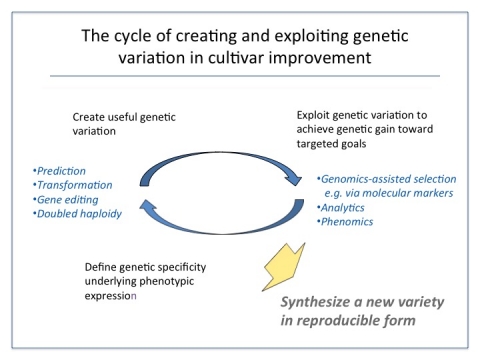
Process to Pipeline
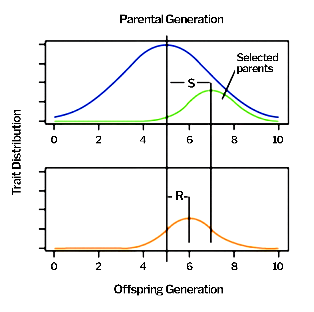
The process is fashioned to increase the frequency of favorable alleles for the traits specified in the product target… and this goal is reflected in the way that parents are chosen, outstanding progeny are identified, and new cultivars are created (Fig. 2). R is selection response, S is selection pressure, and h2 is heritability in the Breeder’s Equation
[latex]R=h^2S[/latex]
and
[latex]h^2 = \dfrac{R}{S}[/latex]
The process is designed to produce a pipeline of improved cultivars, maximizing response to selection (R) and the rate of genetic gain (∆G).
Maximizing Gain
Looking more closely at the equations, R can be written a number of ways:
[latex]\begin{align} R &=ih^{2}\sigma _{p} \\ &= i\dfrac{\sigma^2}{\sigma^2_{p}}\sigma _{p} \\ &= i\dfrac{\sigma_a}{\sigma^2_{p}}\sigma _{p} \\ &= ih\sigma_p \\ \end{align}[/latex]
where:
h2 is narrow sense heritability,
σP is phenotypic standard deviation,
σP2 is phenotypic variance,
i is selection intensity,
σa is additive genetic standard deviation,
σa2 is additive genetic variance, and
h is accuracy of selection (the square root of h2).
And can be expressed as:
[latex]\Delta G=\dfrac{ih^{2}\sigma_{p}}{L}[/latex]
where L is the length of a breeding cycle.
Considerations in Choosing Parents
In choosing parents, consider:
- best performers for traits of interest (i.e. contributors of favorable alleles).
- genetically diverse contributions of favorable alleles (i.e. genetic diversity so as to boost the overall frequency of favorable alleles and the number of loci with the favorable allele present).
Germplasm Banks
Base germplasm can be accessed through the many germplasm banks around the globe. For soybean, there are 189 such repositories, the major germplasm banks listed by the FAO (2010) are listed in Table 1 (extract from Table 2 in Jacob et al, 2016).
| Germplasm Bank | No. Accessions | No. Advanced Cultivar Lines |
|---|---|---|
| ICGR-CAAS (Institute of Crop Germplasm Resources, Chinese Academy of Agricultural Sciences) | 32,021 | n/a |
| SOY (Soybean Germplasm Collection, United States Department of Agriculture, Agricultural Research Services) | 21,075 | 84 |
| RDAGB-GRD (Rural Development Administration National Institute of Agricultural Biotechnology-Genetic Resources Division, Republic of Korea) | 17,644 | 176 |
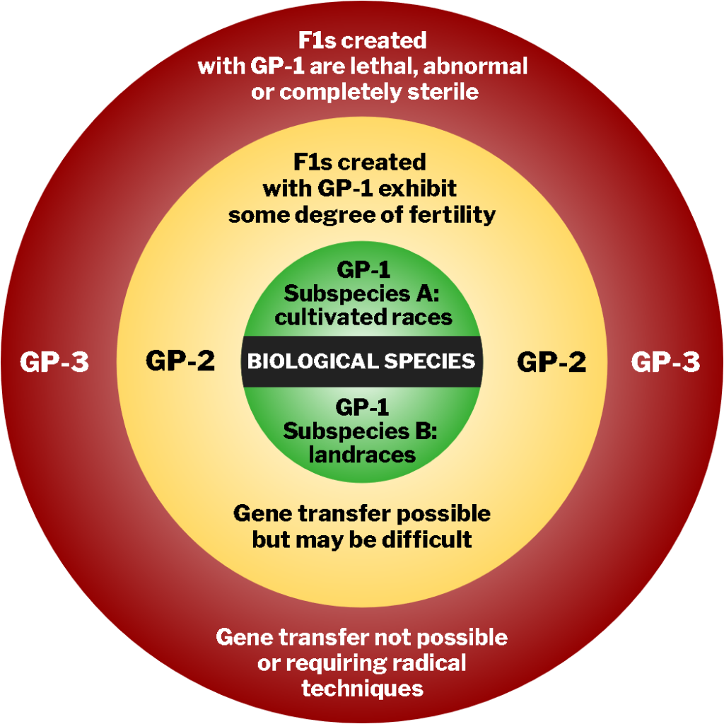
Primary, Secondary, and Tertiary Gene Pools
Germplasm banks may contain materials from the primary, secondary, or tertiary gene pools denoted as GP-1, GP-2, and GP-3, respectively (as defined by Harlan and de Wet, 1971) (Fig. 3).
Sources of Parental Germplasm
Potential sources of parental germplasm include:
- Current cultivars.
- Elite breeding lines.
- Acceptable breeding lines with superiority in one or a few characteristics (e.g., genetic stocks).
- Plant introductions, landraces.
- Related species such as wild relatives.
Which of these source types could be utilized to create a “good x good” cross?
What is a “good x good” cross?
A “good x good” cross is ideal!
Both parents possess favorable alleles for each character, giving a high likelihood that at least some of the progeny will exceed the performance of either parent for each character.
What factors determine that likelihood?
- The expected frequency of desired genotypes in the breeding population for each character.
- The number of traits being selected.
- The inheritance of the character to be improved.
- The number of progeny evaluated.
Favorable alleles contributed by each parent are distinctive (i.e., parents contribute different favorable alleles).
Ideal Parents Possess Favorable Alleles
To determine if prospective parents possess favorable alleles for traits of interest, consider:
- High mean phenotypic performance
- In a self-pollinated crop like soybean, the mid-parent value is the best indicator of performance of progeny from a prospective cross.
- Favorable molecular marker profile (e.g., mapped QTLs)
- Estimated breeding value
Ideal Parental Combinations are Genetically Diverse
To determine if prospective parents are genetically diverse, utilize:
- Pedigree analysis.
- Geographic inference.
- Cluster analysis based on molecular marker profile.
Assessing Genetic Diversity Based on Molecular Marker Profile
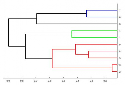
Genetic diversity of prospective parents can be assessed using cluster analysis based on molecular marker profiles.
Lines are genotyped for a set of markers and marker alleles are scored. Each pair of lines is compared for each marker locus to compute an overall estimate of similarity, which is later converted to an estimate of dissimilarity.
Cluster analysis provides a visual depiction of the relative dissimilarity among the lines, which is referred to as a dendrogram (Fig. 4).
Tips for Cluster Analysis
In performing cluster analysis based on marker data:
- Consider the type of marker to sample the genome and the number of markers needed for adequate coverage.
- Choose a method for estimating dissimilarity.
- Choose a method for joining clusters.
- Include some familiar lines of known background in the analysis to serve as “anchors”.
- Remember that the output is relative to the lines included in the analysis, not absolute.
Clustering Based on Pedigree Records
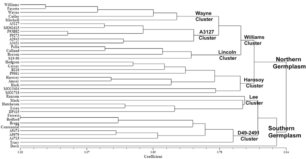
Cluster analysis can also be used to represent genetic diversity graphically, based on complete and accurate pedigree records. The genetic diversity of 38 soybean lines prominently used as parents to develop the current U.S. commercial soybean germplasm base is depicted in the dendrogram below. The results are from cluster analysis based on dissimilarity estimates computed from the coefficient of parentage (Fig. 5).
Suitable Parents for a Stated Product Target
Consider the following product target…
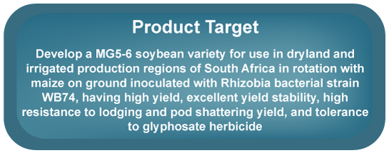
The product target can be dissected to specify the desired characters, their measurement standards, and threshold levels. For example, Table 2 below.
| Characteristic | Measurement Standard | Threshold Level/Range |
|---|---|---|
| High seed yield | Machine harvest; seed weight at 13% moisture basis; expressed per unit of land | 10% greater than Variety X |
| High yield stability | Use regression analysis or GGE biplot analysis |
Comparable to Variety X |
| Lodging resistance | 1-5 scale: 1=plant erect, 5=prostrate | Score ≤ 2 |
| Resistance to pod shattering | Oven dry method; 10 point scale measuring percentage affected: 0=none, 1=1-10%, 10=91-100% | Score ≤ 1 |
| Medium maturity | Maturity Group; day length & temperature requirement to initiate floral development; full range includes Group 000 to Group 9 | MG 5-6 |
| RR1 Event (Roundup Ready 1) | Integrate 40-3-2 | Pre-determined level of glyphosate tolerance |
Describe the characteristics of parents comprising a “good x good” cross to begin New Line Development in terms of:
- Types of germplasm.
- Traits exhibited in each prospective parent and levels of each trait.
What if the ideal parental combination is not feasible?
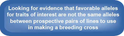
Assessing Prospective Parents for Favorable Alleles
Whereas cluster analysis highlights genetic diversity, it is not an indicator of favorable alleles for the traits of interest in the prospective parents.
Mean performance provides insights as to whether favorable alleles are present… what we really want to know is the breeding value of prospective parents.
Parents pass on their genes, not their genotype or phenotype, to their progeny.
Breeding Value Defined
Breeding value (BV) is…
- The value of an individual, judged by the mean value of its progeny.
- The value of genes, not genotype, passed on to progeny.
- The sum of the average effects of genes in an individual.
Falconer (1989) defines BV as the mean deviation from the population mean of individuals who received that allele from one parent, the other allele coming at random from the population.
On a single locus example, the sum of the average effect of alleles:
If A1 = 10 and A2 = –10
then BV of A1A1 = 20
BV of A1A2 = 0
BV of A2A2 = –20
Estimated Breeding Value
Estimated breeding value (EBV) is a function of narrow sense heritability (i.e., only additive genetic variance is included).
[latex]EBV=h^2P[/latex]
Phenotype (P) is expressed as deviation from the population mean (µ).
Example:
If P = +3.0 units (i.e. standard deviations) and h2 = 0.33,
Then EBV = +3.0 x 0.33 = +1.0 unit
EBV Predicts Progeny Performance
Estimated breeding value is…
- A statistical prediction of the relative genetic merit of individuals as parents.
Crow (1986) explains that the predicted phenotype of the progeny is the average of the breeding values of the parents.
- Used to rank available candidates for use in developing new breeding populations.
- Computed through methods such as:
– BLUP (Best Linear Unbiased Prediction).
– GS (Genomic Selection).
Best Linear Unbiased Prediction
Best Linear Unbiased Prediction = BLUP
- Best: Minimum error.
- Linear: Estimates are linear functions of the data.
- Unbiased: The average value of the estimate is equal to the average value of the quantity being estimated.
- Prediction: Estimates of random effects are typically referred to as ‘predictors’ (estimates of fixed effects are called ‘estimators’).
Origin of BLUP
BLUP originated in animal breeding, where choice of parents is critical to maximizing the use of an expensive sire. The progeny resulting from the breeding cross live for years and comprise the herd.
In plant breeding, we choose many breeding pairs and we can discard any breeding populations we don’t like!
BLUP Model
Phenotype = Environmental Effects + Genetic Effects + Residual Effects
[latex]y_{ij} = \mu_i + g_i + e_{ij}[/latex]
where:
[latex]y_{ij}[/latex] is the [latex]jth[/latex] record observed for the [latex]ith[/latex] line
[latex]\mu_{i}[/latex] is the identifiable nonrandom (fixed) environmental effects such as year, location
[latex]g_{i}[/latex] is the sum of the additive, dominance, and epistatic effects of the ith line
[latex]e_{ij}[/latex] is the sum of the random environmental effects from the [latex]jth[/latex] record of the [latex]ith[/latex] line
Partitioning Additive Effects
Partitioning the additive effects from the total genotypic effects, the model can be written as:
[latex]y_{ij} = \mu_i + (g_a)_i + (g_d)_i + (g_e)_i + e_{ij}[/latex]
[latex]y_{ij} = \mu_i + (g_a)_i + e^{*}_{ij}[/latex]
with [latex]e^{*}_{ij}[/latex] including all nonadditive genetic effects as well as error.
Dealing With Fixed Effects
The concept of “fixed effects” stems from the principle of fair comparisons. Although phenotypes and breeding values are often expressed as deviations from group means, it is desirable to make comparisons on an equitable basis.
For example, it would not be fair to compare yields in a wet year to yields in a dry year.
To compare individuals on a comparable basis, phenotypes are adjusted for known fixed effects.
The Mixed Model Equation
The mixed model equation partitions fixed and random effects:
[latex]Y=X\beta+Z\mu+e[/latex]
where:
[latex]Y[/latex] = the vector of observed values,
[latex]\beta[/latex] = the vector of fixed effects,
[latex]\mu[/latex]= the vector of random genetic effects (the EBVs),
[latex]e[/latex] = the vector of residuals (error),
[latex]X[/latex] and [latex]Z[/latex] are design matrices that relate elements in [latex]\beta[/latex] and [latex]\mu[/latex] to elements in [latex]Y[/latex].
Thus, both breeding values and fixed effects can be estimated.
Solving the Mixed Model Equation
To estimate BVs, solve for:
[latex]\begin{pmatrix} X'X & X'Z \\Z'X & Z'Z+A{^{-1}\alpha}\end{pmatrix}\begin{pmatrix}\beta\\\mu\end{pmatrix}=\begin{pmatrix}X'Y\\Z'Y\end{pmatrix}[/latex]
where:
[latex]A^{-1}[/latex] is the inverse of the matrix of genetic relationships among individuals and,
[latex]\alpha[/latex]=[latex]\frac{(1 - {h}^2)}{h^2}[/latex] where [latex]{h^2}[/latex] is the narrow-sense heritability for the trait under analysis.
Note: Molecular markers can be used to estimate genetic relationships among lines (instead of pedigree information).
Advantages of BLUP over Mid-Parent Value
In work by Panter and Allen (1995), BLUP was more effective than mid-parent value (MPV) for identifying superior parental combinations and demonstrated higher probability of producing superior progeny.
One clear advantage of BLUP over MPV is that the potential of a particular pair of lines as parents could be predicted with BLUP even when no performance data on the lines was available, only performance data on relatives of the lines was available.
For more information, see: Panter, D.M., and F.L. Allen. 1995. Using Best Linear Unbiased Predictions to Enhance Breeding for Yield in Soybean: I. Choosing Parents. Crop Science 35: 397-405.
Advice for Use of EBVs
Tips for use of EBVs:
- EBVs are best used as one piece of information along with all the rest of the knowledge base about prospective parents.
- EBVs are strictly a function of the data used to generate the estimates. You may wish to add new phenotypic data as available (more locations, more years, more related lines) and rerun BLUP.
To distinguish BV from genotypic value:
Breeding value is the expected phenotype of an individual’s progeny and includes only additive effects, whereas
Genotypic value is the expected phenotype of an individual given its genotype; includes additive and non additive effects.
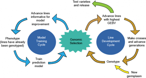
What is Genomic Selection?
Genomic Selection is comprised of methods that use genotypic data across the entire genome to predict performance of any quantitative trait with high accuracy (Fig. 6).
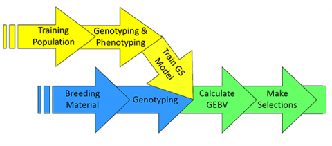
A collection of representative individuals (i.e., Training Population) is phenotyped and genotyped to “train” a model with estimated effects for a genome-dense set of molecular markets for a particular quantitative trait.
Genomic Estimated Breeding Value
How is Genomic Selection applied to choose among prospective parents?
- Estimates of effects are computed for each marker allele using an appropriate training population.
- Genomic Estimated Breeding Values (GEBVs) are calculated for prospective parent lines based on the model. The GEBV is essentially a sum of the effects across the individual’s genome.
- Individuals with the highest GEBVs are used as parents to create the next generation. They are also advanced to varietal testing for possible release as new cultivars, bypassing preliminary testing (Fig. 7).
Use of Suboptimal Parents
So far, we have considered the scenario when two elite lines are suited as parents to supply favorable, diverse alleles for the traits specified in a product target. This is the ideal.
Now, let’s examine the situation where you are not able to work with a “good x good” cross.
What are some of the reasons why suboptimal crosses may be the only option available to accomplish a particular product target?
Moderating the Effect of a Non-elite Parent
With a “good x not-so-good” cross, the breeder can modulate the effect of the non-elite parent through backcrossing to the elite parent before creating progeny for evaluation.
This can take different forms:
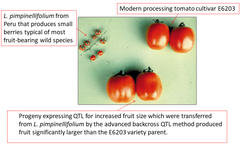
1-3 backcrosses to the elite parent to access potentially favorable genes for a quantitative trait from a lesser elite line, a genetic stock, an elite but unadapted cultivar, or a wild relative (Fig. 8).
≥6 backcrosses to introgress a single gene into an elite cultivar to create an isoline that performs equivalently in every way as the elite parent except for the integrated new trait (e.g., trait integration with disease resistance) (Fig. 9).
The Role of Backcrossing
Backcrossing (ahead of self-pollination) allows the breeder to determine the desired “dosage” of the non-elite parent genome.
With each repeated crossing to the recurrent parent (i.e. elite parent), the amount of germplasm from the non-recurrent parent (i.e. non-elite parent) is reduced by half (Fig. 10).
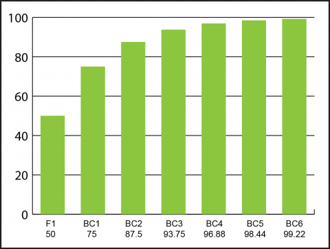
[latex]\%RP(n)=1-\left( \frac{1}{2} \right)^{n+1}[/latex]
where:
[latex]\%RP[/latex] is the percentage of recurrent parent germplasm recovered, and
[latex]n[/latex] is the backcross generation number.
Choice of Parents Affects Choice of Breeding Methods
If a suboptimal cross is the only available option to meet a specific product target, the approach to breeding strategies will look different than the ideal situation where two elite parents can provide the favorable alleles needed.
Bottom line: Choice of parents affects the choice of breeding methods!
Types of Parental Crosses
Although 2-parent combinations are the most widely used, breeding populations can be developed using multiple parents. For example:
- A 3-parent breeding population is formed by mating a 2-parent population to a third parent:
(P1 x P2) x P3. The plants of the 2-parent population may be at F1 (as indicated by this pedigree)
or some later stage of inbreeding. - A 4-parent population, often referred to as a “4-way cross”, can be formed in two ways:
- (P1 x P2) x (P3 x P4) where each parent contributes ~25% of the alleles
- [(P1 x P2) x P3] x P4 where P1 and P2 contribute ~12.5% germplasm, P3 contributes ~25%, and P4 contributes ~50%.
- A complex breeding population is formed using >4 parents.
In each case, the “dosage” of each parent is determined by the way the population is formed.
Complex Parental Crosses
A complex breeding population can involve five to hundreds of parents! This comes with advantages and disadvantages (Table 3).
| Advantages | Disadvantages |
|---|---|
The greater the number of parents:
|
Expected mean peformance of the progeny is still the mean of the parents for self-pollinated crops.
If some parents are not elite for traits of interest, performance is not likely to exceed the performance of the best parent for each trait. |
| Greater probability of heterozygosity at multiple loci. | The greater the number of parents, the more generations required for inter-mating, which can lead to significant time expansion of a breeding cycle compared to 2-parent populations. |
| More allelic combinations possible! | Might not be a efficient as multiple 2-parent populations. |
Creating Progeny and Materials for Testing
Mating Design Determines the Selection Unit
After deciding on the parental combinations, the breeder must make decisions about the progeny to be produced and evaluated (Fig. 1). The mating design employed determines the “selection unit.”
Considerations in Choosing a Mating Design
Factors to consider in choosing a mating design:
- Mode of reproduction (mating flexibility).
- Specific objectives
- Understanding gene action
- Developing estimates of genetic variance components and heritability which are necessary to designing the breeding process structure
- Choosing among breeding methods
- Predicting gain from selection
- Making selections and developing an improved cultivar
- Reliability of the estimates.
Rule: use the simplest design which meets your needs.
For self-pollinated crops, full sib designs are common.
Mating Design Details
Specifics to be determined in choosing a mating design:
- Types of progeny (e.g., full sibs, half sibs, doubled haploids).
- Number of types of progeny and scheme for how parents will be organized.
- Total number of progeny.
Mating Design to Estimate Genetic Variance
Estimation of generic variance requires four steps:
- One or more types of progeny developed.
- Progeny evaluated in set of environments.
- Variance components estimated from mean squares in the ANOVA.
- Variance components interpreted in terms of covariances between relatives.
The Case of the 1-Factor Design
With the use of a single type of progeny, the ANOVA includes one component of variance for progeny and one covariance between relatives. The Expected Means Square table provides a way to estimate the component of variance. This estimate can then be interpreted in terms of the covariance of relatives it represents.
For example (Table 4).
| Source of Variation | d.f. | EMS |
|---|---|---|
| Reps | [latex]k-1[/latex] | n/a |
| Progenies | [latex]p-1[/latex] | [latex]\sigma^{2}+k\sigma^{2}_{\small prog}[/latex] [Design component of variance] |
| Error | [latex](k-1)(p-1)[/latex] | [latex]\sigma^{2}[/latex] |
| Total | [latex]n-1[/latex] | n/a |
If progeny are clonally reproduced, then:
[latex]\sigma ^{2}_{prog}=\text{Cov Identical Twins} = \sigma^{2}_{G}[/latex]
If half sib families, then:
[latex]\sigma ^{2}_{prog}=\text{Cov HS} = \frac{1}{4}\sigma^{2}_{A}[/latex]
If full sib families, then:
[latex]\sigma ^{2}_{prog}=\text{Cov FS} = \frac{1}{2}\sigma^{2}_{A}+\frac{1}{4}\sigma_{D}^{2}[/latex]
Other Mating Designs
Mating designs are classified according to the number of factors, parents, and modalities or a combination of these factors (Cockerham, 1963).
Common mating designs of interest:
- 1-Factor design.
- 2-Factor designs can estimate dominance and additive variances:
- Design I: hierarchical, nested
- Design II: factorial design—cross-classified, parents must be inbreds
- Diallel: used to estimate GCA and SCA
- 3-Factor Designs have at least one grandparent in common and can estimate additional variance components (e.g., epistatic)
- Design III: can screen out psuedo-overdominance.
Level of Inbreeding
Another decision involves the level of inbreeding… will selection be initiated with segregating materials or fully homozygous lines?
Evidence to support Early Generation Testing (Fig. 11) is the strong correlation between early generation performance and late generation performance for yield and other quantitative traits, even with lowly heritable traits.
Furthermore, discarding poor-performing progeny early saves testing resources. However, seed supplies may be limited in early generations. Moreover, the use of homozygous lines eliminates “noise” in the data due to segregation and increases selection accuracy.
The trade-off is between producing more accurate estimates of progeny means vs. sampling a larger number of progeny per cross.
Number of Progeny
Consider the number of progeny to produce and test.
What number of progeny must be tested to assure that at least one truly superior progeny will be identified if, in fact, it exists in that population?
General Guidelines for Determining the Number of Progeny
The number of progeny produced per breeding cross depends on trait heritability as well as the expected proportion of truly outstanding progeny in the specific population and the selection intensity applied.
- There should be at least 200 progeny per population for trait of low to medium heritability.
- If genetic diversity is limited (as it is with soybean), you need even more progeny to find unique gene combinations. More than the minimum of 200 progeny per population is needed.
- Note that the commercial soybean program example suggests population sizes upwards of 500 (200-500 are selected after evaluation for some unspecified characteristics, perhaps disease screening or morphology).
- You must consider the number of traits to be improved and the intended selection intensity for each.
Breeding Methods
How will progeny be advanced to produce materials for testing? This ultimately relates to choice of breeding method. Testing will take place in various stages through the process pipeline. Selections made as a result of one stage of testing will be advanced to the next stage, which often involves the next generation. The breeding method is referred to as the “recombination unit.”
Breeding methods involve the progression of selected materials through the breeding pipeline. Since advanced stages of testing are intended to provide a view of performance of entries as released cultivars, the breeding method(s) utilized are also transitioning selected lines to the genetic state required for release as a new, improved cultivar.
Notice the example of a commercial soybean breeding program in Chapter 1 which called for a “modified single-seed descent” breeding method to advance S0 plants to S1. [Example: Commercial Soybean Improvement Program in Chapter 1].
How is this method employed?
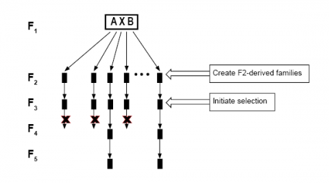
The Pedigree Breeding Method
Single-seed descent is a variation on the pedigree breeding method (Fig. 12), which is a method used in the inbreeding of populations of self- or cross-pollinated species with the goal of developing inbred lines.
The pedigree breeding method typically starts with an F2 population, with self-pollination of each generation until fully inbred lines are generated. Selections can be made in each generation as desired, advancing best families, best rows within a family, or best plants within rows. Thus, the pedigree breeding method can be used to select among families as well as within families.

Single-Seed Descent: A Version of the Pedigree Method
Single-seed descent involves the advancement of F2 lines through self-pollination to homozygosity. This method involves harvesting a single seed from each plant at each generation, bulking the individual seeds, and planting out the entire bulk to represent the next generation. Testing is initiated once the desired level of homozygosity is reached.
This method is an easy way to maintain large populations through the inbreeding process and can be implemented in a relatively short timeframe using off-season nurseries and greenhouses.
Modified Single-Seed Descent
The modified single-seed descent method, referenced in the example of a commercial soybean breeding program, calls for retaining a single pod containing two to three seeds from each F2 plant (instead of a single seed) and bulking across the population. This modified method serves to expand the number of F2:3 families represented in the breeding population.
Evaluation and Selection
Evaluation and Selection
The cycle of cultivar improvement and, thus, the process of cultivar development (Fig. 1) embodied by the process pipeline, centers on the product target. Genetic variation represented in the breeding populations is exploited to make genetic gain toward the defined product target.
Having decided what materials to evaluate, the next key decisions involve:
- the basis for evaluation.
- how the evaluations are conducted, and
- criteria for selection.
The key is to focus on these to maximize the ability and probability of identifying outstanding individuals that meet or exceed the product target if these are present in the breeding populations!
Trait Screens
Screens are needed to measure traits of interest.
[latex]\dfrac{t}{ha}=\dfrac{\text{shelled seed weight (in kg)}}{plot}\times\dfrac{100-\text{%mst}}{87}\times\dfrac{1 t}{1000 kg}\times\dfrac{\text{number of plots}}{ha}[/latex]
With soybean, seed yield is adjusted to a standard 13 percent grain moisture and expressed in weight per land unit.
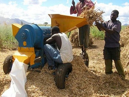
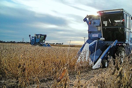
For example, seed yield in soybean is typically measured using a seed thresher (Fig. 13, above) or a combine (Fig. 14) based on weight of the seed per plot.

Seed moisture may be measured using a moisture meter (Fig. 15). Typically, the moisture meter is incorporated in the combine to simplify data collection.
The Need for Protocols
Protocols are needed to ensure that trait measurements are performed accurately, uniformly across the entire experiment, and in conformity with accepted practices.
Note that with the soybean product target example, there is a need for a protocol to describe in detail the exact procedure to use in evaluating pod shattering (also called pod dehiscence).
Romkaew and Umezaki (2006) confirmed that the oven-dried method is a reliable way to discriminate between cultivars that are resistant and susceptible to pod shattering.
METHOD: 30 pods, each with 2 seeds, which have been maintained at <50% relative humidity, are exposed to 60ºC in an oven for 7 hours. The number of opened pods is counted and the percentage of pod shattering is computed.
Crop Ontology
Wait, there’s more…
The performance measurement must be expressed in terms of a scale known to the Community of Practice for the particular crop. Uniform nomenclature is important to sharing information and results, whether internal to the breeder’s organization or to the plant breeding community at large.
The BMS (Breeding Management System) features an ontology for a number of crops.
Choice of Testing Sites
What is the relationship between the testing locations and the market region?
Testing locations are intended as “samples” of the market region. Therefore, it is essential that all the elements of the production areas in the market region are represented and reflected in the characteristics of the testing locations:
- Geographical position.
- Season (if there is more than one per year).
- Soil type.
- Planting dates.
- Cultural practices of farmers in the region: tillage, fertilizer regimes, harvesting methods, irrigation, microbial inoculation of the soil, crop rotation, etc.
Ideal testing locations represent the market region well, and they also enable discrimination among test entries (i.e. differences among test entries are apparent). The uniformity (lack of variation) within a test site allows for the variation in performance among test entries to be front-and-center.
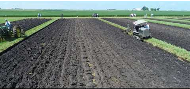
Field Uniformity
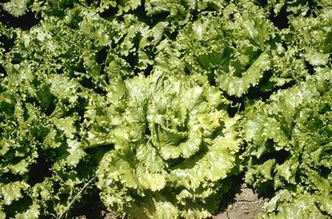
For testing sites, choose fields that are uniform (Fig. 16).
What factors contribute to uniformity?
- Topography.
- Soil type.
- Previous crop.
- Planting preparation.
- Access to moisture.
- Protection from disturbance (if goats get into the field, they probably won’t sample evenly across the field!).
Any differences within a field should be associated with different blocks to the extent possible. For example, confine to one block a low spot in the field that may harbor standing water. That way, the block (and not the whole location) can be discarded if necessary.
Block sizes that are too large result in a lack of uniformity and homogeneity within. The choice of the proper experimental design safeguards the homogeneity of the block. For example, advanced yield trials often include many entries grown in larger-sized plots. Because one block would be too large to maintain homogeneity, an incomplete block design is typically employed to accommodate all and effectively partition any environmental effects.
Appropriate Experimental Design for Trials
Conduct evaluations using appropriate experimental designs to partition variation due to genotype, the environment, and other sources.
Proper execution includes:
- Randomization to guard against bias.
- Replication to capture natural variation among experimental units to be treated alike.
- Use of blocking to partition variation due to environmental influences.
Best Practices in Data Collection
Data integrity must be safeguarded in data collection!
- Prepare to collect data before going to the field or greenhouse. This may mean printing forms for data collection that reflect the field layout. (You do not want to search for the plot number on a form when recording your observed data value.)
- Staff to properly collect data effectively. Having one person to evaluate and another person to write in the observed score on the form can work well. It is best to have the same person rate the entire trial; however, if that is not feasible, assign those ratings to individual reps.
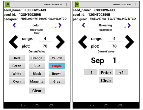
- Data collection programs like Field Book (Fig. 17) may be useful, facilitating data collection on a Kindle or an Android phone.
Traits to Observe and Record
What traits need to be observed and recorded?
Certainly include all the traits specified in the product target. Sometimes, it can be useful to collect data for additional traits, especially those that correlate with target traits.
For example, soybean seed yield is positively correlated with:
- Number of pods.
- Number of seeds per pod.
- Fruiting period.
- 100-seed weight.
Recording correlated traits provides an opportunity to collect additional information on key traits. Furthermore, sometimes it is much more feasible to measure a highly correlated trait that may be easier or less expensive to collect, or that can be collected earlier in the crop life cycle, shortening the breeding cycle.
Indirect Selection
Evaluation and selection based on a correlated trait is an example of indirect selection.
To improve Character X, we might select for another Character Y. In this case, Character Y is considered a “secondary trait.”
What is the expected response to selection in Character X when selection is applied to Character Y?
The expected correlated response of X when selecting based on Y is:
[latex]CR_X=ih_Xh_Yr_{G_Xy}\sigma_{P_X}[/latex]
Given that the response of Character X selected directly is:
[latex]R_X=ih_X\sigma_{A_X}[/latex]
Indirect selection will result in relatively greater genetic gain for Character X than direct selection, if:
[latex]r_{G_Xy}h_Y>h_X[/latex]
Examples of Secondary Traits
Some examples of secondary traits used in crop improvement include:
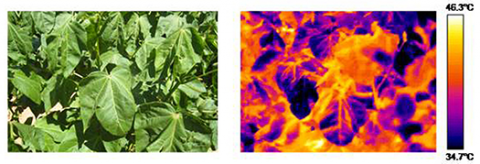
- Canopy temperature as a proxy for drought stress tolerance (Furbank and Tester, 2011) (Fig. 18).
- Root mass under water-limited conditions as a proxy for drought stress tolerance.
- Leaf senescence below the ear as a proxy for low nitrogen tolerance in maize (Banziger and Lafitte, 1997).
- Yield component characteristic (e.g., 100-kernel weight) as a proxy for grain yield.
Choosing Secondary Traits
In choosing secondary traits, consider those that:
- Correlate genetically with the trait of interest in the given target market environment.
- Have higher heritability than the trait of interest (less non-additive genetic variation),
preferably above 0.6. - Exhibit genetic variation.
- Are not associated with poor performance in non-stressed environments.
- Easily, cheaply measurable (need a good screen!).
- Can be measured on a per-plant or per-plot basis, preferably in a non-destructive manner.
Ancillary Traits
There may be other instances where you wish to collect traits other than those in your product target.
- If you wish to estimate harvest index, calculations involve the “seed yield to biomass” ratio. Therefore, biomass must be measured.
- Other characteristics may be collected to gather and present information in order to categorize potential new cultivars. For instance, soybean characteristics typically collected to help position any prospective new cultivars appropriately in the marketplace include:
- Presence of pubescence.
- Seed coat color (16 categories).
- Hilum color.
- Growth type: determinate or indeterminate.
Thus, you may have good reason to expend the time, effort, and resources to measure, record, and analyze other traits, besides those in the product target, to help identify outstanding progeny that may be prospective improved cultivars.
Consider all your data needs before implementing the trial.
Multiple Trait Selection
Product targets are never about a single trait. Typically, plant breeders seek to develop cultivars improved for a number of traits. Let us look at different ways we can approach selection considering that our product target involves multiple traits.
Multiple-trait selection approaches include:
- Tandem selection.
- Independent culling levels.
- Index selection.
Tandem Selection
Tandem selection is a methodology involving selection for one trait at a time (Fig. 19). Selection for each trait is sequential; selection thresholds and selection intensities for each trait are independent. The shaded area indicated the selected individuals in the population.

Tandem selection is a common practice. It is often deployed for traits that affect adaptation or involve stress tolerances.
Examples:
- Tropical maize populations which may be used for improving temperate maize have been selected for photoperiod sensitivity prior to selection for traits such as yield.
- In elite materials, selection for disease resistance may precede selection for yield.
Independent Culling Levels
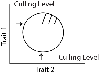
Independent culling is a method involving selection for more than one trait in a single step (Fig. 20). Thresholds are established for each trait and only those individuals that meet all trait thresholds are selected. With this method, individuals can be culled on the basis of a single trait without having to wait for or even collect observations of the other trait(s).
Index Selection
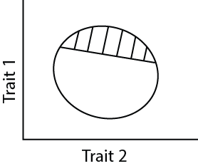
Index selection is a method involving selection for more than one trait simultaneously on the basis of a single index value (Fig. 21). It accounts for the relative superiority of individuals for all of the traits included in the index.
The selection index is usually a linear function of the various traits involved. Each trait is weighted according to its importance. Furthermore, the index typically takes into account the genetic correlation between pairs of traits so that progress can be made even with negatively correlated traits.
Smith-Hazel Index
Index selection is a form of indirect selection. As for selection indices, there are a number of types. All are based on the original index independently developed by Smith (1936) and Hazel (1943).
The Smith-Hazel Index takes the form:
[latex]I=b_1X_1+b_2X_2+...+b_nX_n[/latex]
[latex]I=\sum{}b_iX_i[/latex]
where:
[latex]b_i[/latex] is the weight of trait i,
[latex]X_i[/latex] is the phenotypic value for trait i.
[latex]i[/latex] is calculated for each individual in the population. The index value becomes the new variable upon which breeding progeny are evaluated. Individuals with the highest values are selected.
Weights in the Smith-Hazel Index
How are weights calculated when using the Smith-Hazel index?
Weights take into account the phenotypic and genetic covariances among the traits, as well as the economic value of each trait. Weights can be calculated by solving the following equation:
[latex]b=P^{-1}G_a[/latex]
where:
[latex]b[/latex] is an [latex]nx1[/latex] vector of the [latex]b_i[/latex] values,
[latex]P^{-1}[/latex] is the inverse of the [latex]nxn[/latex] matrix of phenotypic covariances among the traits,
[latex]G[/latex] is the[latex]nxn[/latex] matrix of genetic covariances among the traits,
[latex]a[/latex] is an [latex]nx1[/latex] vector of economic weights for the traits.
Note that [latex]G[/latex] and [latex]a[/latex] may be difficult to estimate.
See Quantitative Genetics: Multiple Trait Selection (coming soon!) for more on index selection.
Efficiency in Selecting for Multiple Traits
Which multiple trait selection approach is most effective?
According to Hazel and Lush (1942) the order is:
Selection index > Independent culling > Tandem selection
Testing Regime
To facilitate selection, the pipeline process embodies a testing regime to evaluate progeny, resulting from the various breeding crosses, for all the traits of interest.
Let’s review the testing regime outlined in the Commercial Soybean Improvement Program example that was introduced in Chapter 1:
| Season1 | Activity |
| Winter 0 | Make breeding crosses |
| Summer 1 | Self or BC each population |
| Winter 1a2 | Grow 200 F2 or BC1 populations (i.e. S0 generation) that have been formed in previous years
Advance the S0 plants to the S1 generation by a modified single-seed-descent method, retaining single pod (instead of a single seed) with 2-3 seeds; bulk by population |
| Winter 1b | Plant S1 seed bulk;
Select 200-500 plants (~350 per population) and save selfed (i.e. S2) seed |
| Summer 2 | Yield trials for 70,000 S2 families (across all populations) in unreplicated trials at 1-2 locations;
Select the best 5,000 based on yield performance; Save S3 seed from the trials |
| Summer 3 | Yield trials for 5,000 S3 families at 3-5 locations;
Select the best 200 based on yield performance; Save S4 seed from the trials |
| Summer 4 | Yield trials for 200 S4 families at 15-25 locations;
Select the best based on yield performance; code selected as ‘experimental’ lines; Save S5 seed from the trials |
| Winter 4 | Increase seed of experimental lines |
| Summer 5 | Yield trials of experimental lines at 20-40 locations
On-farm strip tests (i.e.150-300 m2 plots) at 20-100 locations |
| Summer 6 | Yield trials of ‘advanced’ lines at 20-50 locations On-farm strip tests (i.e. 150-300 m2 plots) at 30-500 locations |
| Fall 6 | Release 0-5 new varieties |
1Summer represents the main growing season, winter denotes off-season activities; number after season indicates the year in the development pipeline
2Winter nurseries may be grown back-to-back in the same winter season
Aspects of the Testing Regime
As noted earlier, this example serves a market region with one growing season, which is referred to as “Summer.” “Winter” designates off-season activities.
We observe the following with respect to the testing regime:
- The main focus of testing is grain yield in this example (no other trials other than yield trials are mentioned, although selection among individual S1 plants is indicated). High grain yield is obviously the trait of the utmost priority in producing new varieties (in this case).
- A large number of breeding populations are created.
- Yield trials are initiated with a very large number of S2 families and continue every growing season in the market region.
- Selection intensities are high (only a small proportion of the tested families are advanced to the next generation of testing).
- The number of locations for yield testing increases as the number of tested families decreases.
- Lines that are selected after Summer 4 yield trials (third year of yield testing) are coded as “experimental” and progressed to wide-area testing the following growing season. Lines that continue to meet or exceed product targets are progressed to “advanced” line status in further wide-area testing.
- Wide-area testing includes “on-farm trials” managed by potential seed customers. Wide-area testing could also include National Performance Trials required for the registration of a new variety.
- Overall, there are at least five years of comprehensive performance testing: five seasons of “research” yield trials, and two seasons of wide-area testing which are initiated after three seasons of research yield trials.
- Because soybean is a predominantly self-pollinated crop (pollination typically takes place before flowers open), seed for planting the following year’s trials can be retrieved from yield plots (after recording yield measurements). Seed production for wide-area trials that require significant seed amounts is done during the off-season to save time.
Testing Progression
Let us examine the progression of testing in the example program.
Preliminary yield trials are conducted in Summers 2 and 3. Preliminary yield trials are characterized by a large number of entries observed at a small number of locations.
In the example program, there is a third year of yield testing with only a fraction of the number of lines originally created (i.e. 200 S4 families).
Trials are unreplicated, meaning that there’s only one rep of the test at each location.
The testing regime takes into account the various factors contributing to phenotypic variation so that variation associated with “genotype” can be partitioned and differences between entries can be perceived.
We know that:
[latex]V_P = V_G + V_E + V_GxE +error[/latex]
[latex]and[/latex]
[latex]V_E = V_n + V_r + V_L + V_Y[/latex]
where:
VP is phenotypic variation
VG is genetic variation
VE is environmental variation
VGxE is variation due to the interaction between genotype and environment
Vn is variation among plants in an experimental unit (e.g. plot)
Vr is variation among replications of experimental units
VL is variation among locations
VY is variation among years.
These formulas indicate that, to elucidate variation due to genotypic variation, variation due to environment must be accounted for and error must be well controlled.
To accomplish this, the example demonstrates the following:
- Experimental units containing more than one plant are employed, especially in measuring a low- to medium-heritability trait like grain yield.
- Multiple locations are needed to sample an increasing range of the target market as testing progresses.
- Multiple years (i.e. seasons) of testing are needed to ensure an adequate sample of climatic conditions in the market region.
The regime in the example program also allows for an assessment of GxE (Genotype by Environment interaction). Ideally, a new improved cultivar will perform best or among the best across the entire market region.
Unreplicated Yield Trials
Why does the example program advocate unreplicated yield trials? Isn’t replication needed to identify Vr (i.e., variation among experimental units treated the same)?
Not necessarily. Work by Melchinger et al. (2005) showed that, for a given number of observations of each entry, maximum gains from selection are facilitated by maximizing the number of locations at the cost of replication within locations (Fig. 22). In other words, single-rep trials at more locations provide the greatest opportunity for gains in grain yield for any case where there are two or more locations involved. Note that two locations with one rep each facilitate more genetic gain than selection based on one location with two replications.
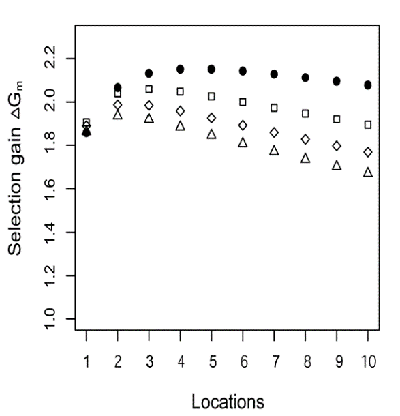
Symbols indicate the number of replications: [latex](r):r=1(\bullet)[/latex], [latex]r=2 (\square)[/latex], [latex]r=3 (\Diamond)[/latex], [latex]r=4 (\bigtriangleup )[/latex].
Early Generation Yield Testing
In Summer 2, there are 70,000 S2 families grown at 1-2 locations. Only the best 7% will be advanced to the next yield trial.
What is the genetic state of these testing materials? Are these lines fully inbred, or is there some level of heterozygosity present?
Click here to reveal the answer
The S2 lines are F4 equivalents and, therefore, are not fully homozygous. On average, they are 87.5% homozygous.
This is an instance of early-generation testing.
Experimental Designs Employed
Overall, there are at least five years of comprehensive performance testing: five seasons of “research” yield trials, and two seasons of wide-area testing which are initiated.
What experimental designs would be suitable for the various stages of yield testing?
Research trials feature:
- 70,000 entries in Summer 2
- 5,000 entries in Summer 3
- 200 entries in Summer 4
In Summers 5 and 6, research trials continue. Only a small number of entries are still being advanced from previous trials. However, the type of testing done in Summers 5 and 6 is very comprehensive coverage of the market area. This testing is meant to provide a good sampling of the types of environments that would be encountered should one or more of these lines be released as a new variety. These tests would include other entries besides the advanced selected lines from the particular breeding crosses represented in Winter 1a. These tests may include a broad set of current cultivars, competitive cultivars, advanced lines from previous years, etc. Therefore, these tests are likely to include more than 30 entries overall.
Suitable Experimental Designs
Suitable experimental designs are those that facilitate accurate and precise estimates of mean performance, even with a large number of entries.
Incomplete block designs are suitable because they partition a replication of the full experiment into smaller, more homogeneous units of land. (Note: with a large number of entries, one full set of entries is likely to occupy a large space in a field, making it difficult to maintain homogeneity over this large area.)
You may be familiar with these types of incomplete block designs:
- Lattice
- Alpha-lattice
- Row-column design
These are commonly used in yield testing when trials include a large number of entries.
Furthermore, within the context of these types of experimental designs, augmented designs can be considered as a means to increase precision with unreplicated trials.
Would incomplete block designs also be suitable for conducting the on-farm trials? Why or why not?
Click here to reveal the answer
Yes, incomplete block designs are suitable for farmer-participatory trials, although with increased plot sizes, block sizes would be smaller.
Augmented designs would be a good fit as well.
Number of Locations
In the example program, the number of locations (i.e. environments) expands each year of testing… and a range for the number of locations at each point of progression in testing is given.
What criteria factor into the determination of the number of locations?
In the example, Summers 2 and 3 are winnowing down the number of overall entries to a manageable number, which will be screened in Summer 4 to assess the magnitude of yield differences among the lines and the lines compared to check entries. The number of locations is ramped up as the number of entries is pared down. Budgets are an important consideration in determining the number of locations for these seasons.
Summer 4 represents the critical assessment of the remaining lines for grain yield. The Summer 4 yield trial is critical to identifying lines that meet the stated selection benchmarks. Therefore, the number of locations to be utilized in Summer 4 is pivotal to ultimately determining success in achieving the product target.
Determining the Number of Locations Needed
How many locations are needed to detect a particular Least Significant Difference (LSD)?
The breeder sets the desired probability level (e.g., [latex]\alpha[/latex] = 0.05) and can plug in estimates of the error variance (Verror) and the variance associated with genotype by environment interaction (VGE) obtained in previous trials.
For a two-tailed test with [latex]\alpha[/latex] = 0.05:
[latex]LSD_{0.05}=t_{\alpha/2}\sqrt{2(\frac{V_{error}}{re}+\frac{V_{GE}}{e})}[/latex]
where:
[latex]r[/latex] = number of replications per location,
[latex]e[/latex] = number of locations.
When the number of entries in the trial is large (i.e. >30), the critical value of [latex]t_{\alpha/2}[/latex] is about 2.0.
Thus, the equation becomes:
[latex]LSD_{0.05}=2\sqrt{2(\frac{V_{error}}{re}+\frac{V_{GE}}{e})}[/latex]
The equation can be rearranged to solve for the number of locations required (i.e., [latex]e[/latex] required) to facilitate detection of a certain LSD at the  = 0.05 significance level:
[latex]e_{required}={(\frac{8}{(LSD_{0.05}){^2}}(\frac{V_{error}}{r}+V_{GE})}[/latex]
If the breeder wishes to ascertain a 0.3 t/ha increase in yield, then the equation becomes:
[latex]e_{required}={(\frac{8}{(0.3){^2}}(\frac{V_{error}}{r}+V_{GE})}[/latex]
With unreplicated trials, [latex]r=1[/latex], and the equation can be solved with estimates of the error variance [latex]V_{error}[/latex] and the variance associated with genotype by environment interaction [latex]V_{GE}[/latex] obtained in previous similar trials.
[latex]e_{required}={\frac{8}{0.09}({V_{error}}+V_{GE})}[/latex]
Furthermore, the number of locations can also be determined in the case of replicated trials by plugging in the appropriate value of [latex]r[/latex].
Estimates of Variance Due to Error and to GxE
Note that estimates of error variance (Verror) and the variance associated with genotype by environment interaction (VGE) are easily obtained based on the Expected Mean Square (EMS) terms for the sources of variation (SOV) in the ANOVA. Previous trials of similar size, market area, and trait of interest may be used.
In the following example (n=genotypes, e=environments, and r=replications), genotypes and environments are considered random; the EMS terms are given for pertinent SOV.
| SOV | DF | MS | EMS |
|---|---|---|---|
| Environments (E) | e-1 | n/a | n/a |
| Blocks/E | e(r-1) | n/a | n/a |
| Genotypes (N) | n-1 | MSgenotype | Verror+ rVGE+ reVgenotype |
| GxE | (n-1)(e-1) | MSGE | Verror+ rVGE |
| Error | (n-1)(r-1)e | MSerror | Verror |
| Total | nre-1 | n/a | n/a |
An estimate of [latex]V_{GE}[/latex] can be easily calculated using the mean square for [latex]GxE[/latex] and the mean square error:
[latex]V_{GE}={\frac{MS_{GE} - {MS_{error}}}{r}}[/latex]
Patterns of GxE
Let’s explore further into GxE…
There are three main patterns of GxE exhibited (Fig. 23). Considering performance (y axis) of two cultivars (blue and green lines) at two environments (x axis), GxE pattern may look like this:
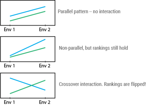
With crossover interaction, the ranking of genotypes is flipped between the two environments. That is, blue is “best” in the first environment whereas green is “best” in the second environment. This makes selection complicated! After all, as plant breeders, we are interested in identifying the “best” genotype for our entire target market if possible.
An ANOVA may indicate the presence of GxE through a statistically significant F-test; however, this does not indicate whether rankings are affected. Further probing is required (e.g., mean comparisons of entries by environment).
Managing GxE
As a plant breeder, there are a number of ways to deal with GxE:
- Ignore it
- Testing done in wide range of environments and selections based on mean performance.
- Does not recognize best cultivars for specific environments.
- Reduce it
- Partition the population of environments into smaller, more homogeneous regions.
- Make selections by region.
- Exploit it
- Reduce GxE by partitioning environments into mega-environments.
- Aims to identify cultivars best suited to specific environments or subsets of environments.
- Also considers “stability” across environments.
What is “Stability”?
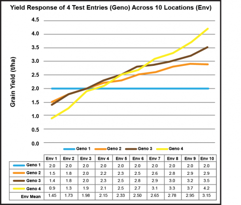
The concept of “stability” involves the performance of a line relative to other lines across a range of environments that represent the target market (Fig. 24). If environments are ranked in terms of their effect (mean performance of all entries) and charted from low to high, the response of the lines tested can be graphed. For example, four soybean lines (i.e. genotypes) are ranked as to their performance for seed yield at each of 10 locations (i.e., environments):
Mean Performance Across Environments as a Measure of Stability
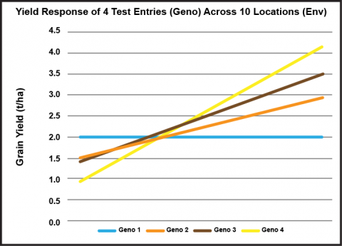
Regression analysis can be implemented to calculate the linear relationship between mean performance and environments for each genotype (bi).
We can examine mean performance as a measure of yield stability (Fig. 25):
- Genotype 1 is constant in its performance across all 10 environments. In this case, bi = 0. Moreover, this entry yielded more than the other lines under less favorable growing conditions.
- Genotype 3 displayed a response similar to the slope of the mean response of all four genotypes across environments (regression not shown).
- Genotype 4 responded best to more favorable environments, displaying its genetic potential. However, it yielded less than the other lines under stressful conditions.
Which genotype exhibits the greatest yield stability?
Deviations From Regression as a Measure of Stability
Although we have examined stability in terms of response across environments, another measure of stability of a genotype can be considered: deviations from the fitted regression line. Excessive deviations from the regression line would suggest erratic response to the range of environments tested.
For more detail on stability analysis, see Bernardo 2010, Chapter 8.5.
Partitioning Environments to Deal with GxE
Another approach to managing/exploiting GxE is to partition environments into homogeneous subgroups or mega-environments. In essence, this leads to the formulation of multiple product targets, one for each mega-environment. Then, testing is conducted accordingly.
Partitioning environments can be facilitated through cluster analysis (the same type of analysis used to partition genetic diversity; (see Choosing Parents) based on data from performance trials across locations and years. Bernardo (2010) offers suggestions on ways to compute distance estimates between pairs of environments.
In Chapter 6 of this course, we will examine a method called GGE Biplot to determine whether a target market region comprises more than one mega-environment. GGE Biplot can also be utilized to assess the stability of tested genotypes.
Advanced Testing
Advanced testing (Summers 5 and 6) focuses on lines that have met or exceeded specifications of the product target in the earlier years of testing (i.e. coded lines). Advanced testing is characterized by:
- Maximal numbers of research testing sites.
- Farmer participation in testing, with larger plot sizes employed to provide a better view of overall performance under real-life field conditions in the market region.
- Wider exposure of farmers to potential new cultivars by maximizing the number of farmer-participatory sites. More farmers have the opportunity to gain experience and familiarization with the potential new products.
The purpose of advanced testing is to confirm coded lines meet or exceed all the specifications in the product target, across an even wider range of samples from the population of environments representing the target market. Furthermore, this testing contributes to the assembly of information for potential product release to farmers for cultivation, and for varietal registration.
Ideally, there is at least one coded line that represents a new “best” for the target market.
Identifying Potential New Products
Potential new cultivars will meet or exceed all the specifications in the product target throughout the entire testing regime. Additionally, such candidate lines will not exhibit any negative characteristics that would make them undesirable to farmers or other stakeholders in the value chain (Fig. 25). Those lines with the best performance overall will be considered for possible release as new, improved cultivars.
According to the soybean breeding pipeline example, zero to five new cultivars may come through as candidates for release. As demonstrated in this chapter, all aspects of the product pipeline are interrelated and require integration for success and value.

If the product pipeline is designed well, integrated fully, and implemented effectively, there is a higher probability that the number of potential new products will be in the 1-5 range. We aim for success!
References
Banziger, M., H.R. Lafitte. 1997. Efficiency of secondary traits for improving maize for low-nitrogen target environments. Crop Sci. 37:1110-1117.
Bernardo, R. 2010. Breeding for Quantitative Traits in Plants. 2nd ed. Stemma Press, Woodbury, MN.
Carmo-Silva, A.E., M.A. Gore, P. Andrade-Sanchez, A.N. French, D.J. Hunsaker, M.E. Salvucci. 2012. Decreased CO2 availability and inactivation of Rubisco limit photosynthesis in cotton plants under heat and drought stress in the field. Environmental and Experimental Botany 83: 1-11. dx.doi.org/10.1016/j.envexpbot.2012.04.001
Cockerham C.C. 1963. Estimation of genetic variances. p. 53- 94. In statistical genetics and plant breeding. National Academy of sciences, NRC.
Falconer, D.S. 1989. Introduction to Quantitative Genetics, 3rd ed. Longman Scientific & Technical, Essex, England.
Fehr, W.R. 1978. Breeding. In A.G. Norman (ed.), Soybean Physiology, Agronomy, and Utilization, p120-155. Academic Press, New York.
Furbank, R.T., M. Tester. 2011. Phenomics – technologies to relieve the phenotyping bottleneck. Trends in Plant Science 16(12): 635-644.
Harlan, J.R., J.M.J. de Wet. 1971. Toward a rational classification of cultivated plants. Taxon 20(4): 509-517.
Hazel, L.N., J.L. Lush. 1942. The efficiency of three methods of selection. J. Heredity 33: 393-399.
Heffner, E.L., M.E. Sorrells, J.L. Jannick. 2009. Genomic selection for crop improvement. Crop Sci. 49:1-12.
Irwin, S.V., R.V. Kesseli, W. Waycott, E.J. Ryder, J.J. Cho, R.W. Michelmore. 1999. Identification of PCR-based markers flanking the recessive LMV resistance gene mo1 in an intraspecific cross in lettuce. GENOME, 42:982-986.
Jacob, C., B. Carrasco, A. R. Schwember. 2016. Advances in breeding and biotechnology of legume crops. Plant Cell Tissue and Organ Culture 127:561-584. DOI 10.1007/s11240-016-1106-2
Melchinger, A.E., C.F. Longin, H.F. Utz, J.C. Reif. 2005. Hybrid maize breeding with doubled haploid lines: Quantitative genetic and selection theory for optimum allocation of resources. Pp8-21. In Proc. 41st Annual Corn Breeder’s School, Mar 2005.
Mikel, M.A., B.W. Diers, R.L. Nelson, H.H. Smith. 2010. Genetic diversity and agronomic improvement of North American soybean germplasm. Crop Sci. 50:1219-1229.
Mumm, R.H. 2013. A look at seed product development with genetically modified crops: Examples from maize. J. Agricultural and Food Chemistry 61(35): 8254-8259. DOI: 10.1021/ jf400685y
Mumm, R.H., J.W. Dudley. 1994. A classification of 148 U.S. maize inbreds: I. Cluster analysis based on RFLPs. Crop Sci. 34:842‑851.
Mumm, R.H., L.J. Hubert, J.W. Dudley. 1994. A classification of 148 U.S. maize inbreds: II. Validation of cluster analysis based on RFLPs. Crop Sci. 34:852‑865.
Panter, D.M., F.L. Allen. 1995. Using best linear unbiased predictions to enhance breeding for yield in soybean: I. Choosing parents. Crop Sci. 35: 397-405.
Rife, T.W., J.A. Poland. 2015. Field Book: An open-source application for field data collection on Android.
Romkaew, J., T. Umezaki. 2006. Pod dehiscence in soybean: Assessing methods and varietal difference. Plant Production Science 9(4): 373-382.
Tanksley, S.D., S. Grandillo, T.M. Fulton, D. Zamir, Y. Eshed, V. Petiard, J. Lopez, T. Beck-Bunn. 1996. Advanced backcross QTL analysis in a cross between an elite processing line of tomato and its wild relative L. pimpinellifolium. Theoretical and Applied Genetics. 92(2):213-224.
Tanksley, S.D., J.C. Nelson. 1996. Advanced backcross QTL analysis: a method for the simultaneous discovery and transfer of valuable QTLs from unadapted germplasm into elite breeding lines. Theoretical and Applied Genetics. 92(2):191-203.
Yan, W. and I. Rajcan. 2002. Biplot evaluation of test sites and trait relations of soybean in Ontario. Crop Sc. 42(1): 11-20.
How to cite this chapter: Mumm, R.H. (2023). Chapter 2. The Process of Cultivar Development: Pure Line Variety. In W. P. Suza, & K. R. Lamkey (Eds.), Cultivar Development. Iowa State University Digital Press.
Phenotypic value of progeny that is equal to the average or mean of the parents.
The average of the performance of the two parents; abbreviated MPV.
The propensity of a soybean pod to shatter during drying, releasing seeds before harvest time.
A line resulting from pre-breeding.
A counterpart to a line, differing only by one allele at a particular locus
The elite line serving as a parent in the initial and subsequent generations of backcrossing. See also non-recurrent parent.
The donor parent; the line serving as a source of favorable gene(s). See also recurrent parent.
The system of developing progeny
Families are lines within a breeding population derived from same plant(s) in a preceding generation (e.g. selected from the same progeny row in the previous generation or descended from the same F2 plant).
Filter to examine and enable assessment of performance for a given trait.
An established standard procedure or code of conduct for carrying out a particular activity.
The physical entity which can be assigned at random to a treatment. It is also the unit of statistical analysis.
Progress with one trait that is associated with progress in another trait, with both traits changing in the same direction.
Selection applied to some characteristic other than the one it is desired to improve.
A term used in the seed industry to indicate the recognized elite status of a breeding population progeny. Typically, coded lines are entered into a wider scope of testing, which may be conducted in two stages of progression. In the first stage, coded lines are called "experimental" varieties; passing this stage, lines are called "advanced" varieties. Even if coded lines don’t make it to commercial release, these may be considered as prospective parents in creating new breeding populations.
Augmented designs, originally conceived by W.T. Federer, feature replicated check varieties arranged in a standard experimental design and unreplicated plots of new varieties to be tested.
Broadly speaking, location stands for "environment;" location is one dimension of "environment." The term could more broadly represent "season/location" combinations.
A check is a test entry used as an experimental control.
(1) A mega-environment is a group of locations that consistently share the best set of genotypes or cultivars across years (Yan and Rajcan, 2002).
(2) Categories of environments within the target market region that consistently share the best set of genotypes or cultivars across years.
