
Chapter 5: Value-added Trait Integration
Rita H. Mumm
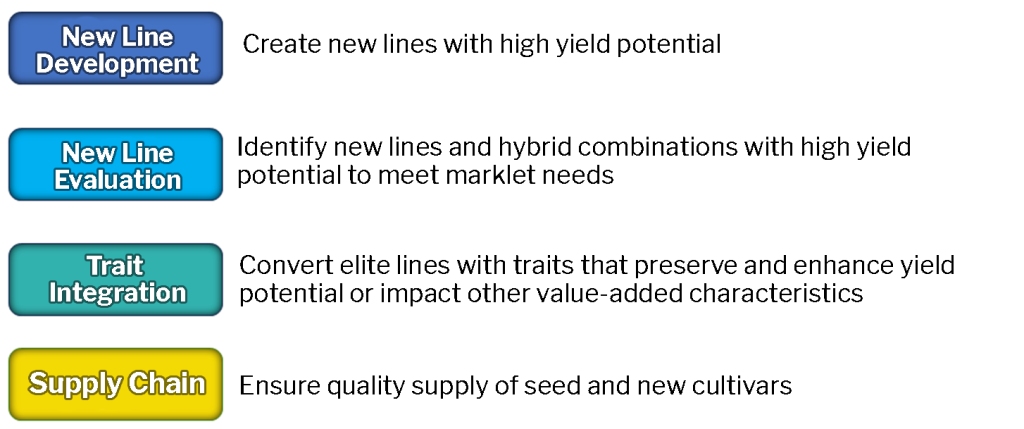
The cultivar development process is comprised of four main functions (as discussed in Chapter 1. Earlier chapters have focused on New Line Development and New Line Evaluation. This chapter will focus on the next step in the product pipeline: value-added trait integration, or “Trait Integration” for short. This core function serves to incorporate high-demand traits to further improve elite cultivars (Fig. 1).
What is a ‘Value-added’ Trait?
A value-added trait (VAT) is a special trait that represents a novel or uncommon characteristic of value to farmers, end-users or consumers when incorporated into an elite cultivar.

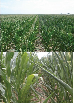
An example in lettuce is resistance to the potyvirus, Lettuce Mosaic Virus (LMV), which causes devastation in lettuce production worldwide and can result in severe crop losses (Fig. 2).
Symptoms vary by variety and timing of infection, yet generally involve deformed heads and discolored leaves. A single, recessive gene, mo1, confers resistance/tolerance.
Think of a VAT as “frosting on the cake!” Typically, it is a “must-have” characteristic for one or more stakeholder groups in the crop value chain, and sometimes such a trait commands a premium price depending on the economics of its deployment.
More About Value-Added Traits
Typically, VATs involve no more than five genetic factors and often are conferred by single genes. Generally, these traits are not common in the gene pool. Some have designated tradenames.
VATs include traits of all types, for example:
- Disease resistance
- Insect resistance
- Herbicide tolerance
- Abiotic stress (e.g., drought tolerance, low fertility tolerance)
- Yield/productivity enhancement
- Nutritional enhancement, e.g., more lysine (corn), healthy oil profile (soybean), reduced lignin content (alfalfa)
- Consumer or end-user preferences, e.g., non-browning (apple), reduced black spot bruising (potato), fruit ripening (tomato)
- Male sterility
- Flower color (rose)
Developing VATs
VATs may be developed through different techniques such as:
- Mutagenesis.
- QTL mapping.
- Transformation (e.g., virus resistant papaya)
- Gene editing (e.g., Sulfonylurea herbicide tolerant canola)
Discussed below are some crop improvement examples through the use of these techniques.
VATs Based on Mutant Genes
Mutagenesis can generate new alleles, some of which may have novel utility in a crop plant.
An example is imidazolinone-herbicide tolerant rice Clearfield® rice developed by BASF. It confers tolerance to a class of herbicides which inhibit amino acid synthesis by inhibiting the acetolactate synthase (ALS) enzyme. The ALS mutant allele was created through chemical exposure to ethylmethanesulfonate (EMS), a mutagen.
Most mutant alleles are recessive, which has implications for product development. For example, for threshold expression of the trait in a hybrid cultivar, two copies of the mutant allele would be required. This demands that both inbred parents of the hybrid carry the allele.
TILLING
TILLING (Targeting Induced Local Lesions IN Genomes) provides a practical path to discovery of single-nucleotide mutations. TILLING is a reverse genetics approach; that is, gene function is determined by analyzing the phenotypic effects of specific engineered gene sequences. Reverse genetics seeks to learn what phenotypes arise as a result of particular genetic sequences. In contrast, forward genetics seeks to understand the DNA sequence that gives rise to a particular phenotype.
Approaches to determining gene function:
- Forward genetics: Determine the DNA sequence that code for the known phenotype.
- Reverse genetics: Determine the phenotype that will be produced from DNA sequence.
Steps in TILLING
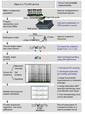
Till et al. (2004) lists steps to finding changes in specific genes of interest (Fig. 4):
- Identify specific genes of interest; target DNA regions to screen
- Create primers to PCR target regions
- Apply mutagen (e.g. ethylmethanesulfonate [EMS]) to pollen or seed
- Screen for mutations in M1 (if from pollen) or M2 generation (if from seed)
- Identify, sequence, and phenotype mutant individuals.
The process has been improved and continues to be optimized (Fig. 4).
VATs Based on QTL
Some VATs are the result of QTL mapping in which native genes have been tagged by molecular markers. Examples include:
- Optimum AQUAmax® corn hybrids by DuPont Pioneer (now Corteva Agriscience) which are drought tolerant. Chromosomal segments identified through marker-assisted breeding to withstand water stress are assembled and deployed. (Knowledge of specific genes [quantity, function, modes of action] is not necessary.)
- AgrisureArtesian one of Syngenta Artesian™ drought tolerant corn hybrids. To develop this VAT, candidate genes associated with water-deficiency stress tolerance were identified through genomics. This led to the discovery of maize genes that protect the plant from drought stress in several different ways, responding to water-deficiency stress with multiple modes of action and at various stages of growth through the corn lifecycle. The genes were validated and pyramided in elite hybrids to deploy the trait (Fig. 5).
VATs Based on Transformation
VATs developed through transformation (also referred to as genetically modified or GM traits) have primarily involved protection of the genetic yield potential of elite cultivars against weed, insect, and disease pests. By and large, these VATs represent novel traits that are either not accessible in the current host species gene pool or which have resulted from the modification of host species genes for expression at higher thresholds, in specific tissues, at certain timing in the host species life cycle, or for silenced expression.
Transformation produces a transgenic event, which becomes the original source of the VAT. An event is defined by the unique DNA sequence inserted in the host genome through transformation and the precise point of insertion. Each event originates as a single plant (referred to as a T0 plant) which was regenerated from a single transformed cell.
Examples of Transgenic VATs
Examples of VATs developed through transformation among others include insect resistant corn and virus resistant papaya:
- YieldGard® developed by Monsanto Company, confers resistance to Lepidopteran insect pests that feed on leaves, stalks, and ears in corn.
- Papaya resistant to Papaya Ringspot Virus (PRSV) was introduced in Hawaii USA in 1998 and was rapidly adopted by Hawaiian growers. Resistance, developed by then Cornell University researcher Dennis Gonsalves, is conferred through gene silencing in response to a virus coat protein gene fragment, Event 55-1. The most commonly grown cultivars are Rainbow, Sunrise/Sunup, Kapoho (Solo), and Kamiya/Laie Gold.
Rapid Adoption of GM Crops
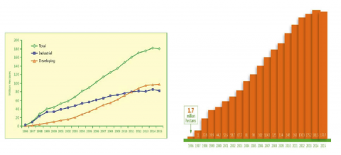
From 1995, when GM crops were first commercialized, through 2015, the land area around the globe planted to GM crops increased from 1.7 million hectares to 179.7 million hectares, making this technology the most rapidly adopted in modern agriculture (Fig. 6).
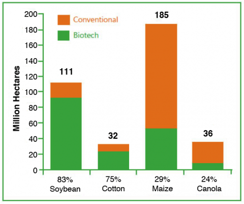
The primary GM crops globally are soybean, maize, cotton, and canola (Fig. 7).
GM Crop Adoption in Africa
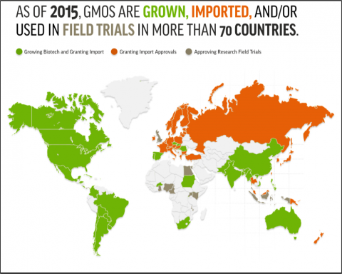
GM crops are widely grown and used throughout the world. In Africa, three countries have approved at least one type of GM crop: Burkina Faso (cotton), Sudan (cotton), and South Africa (maize, soybean, cotton). Others have approved research field trials: Cameroon, Egypt, Ghana, Kenya, Malawi, Nigeria, and Uganda (Fig. 8).
For more on the status of biotech crops in Africa, check out this video by ISAAA.
Stacked GM Traits
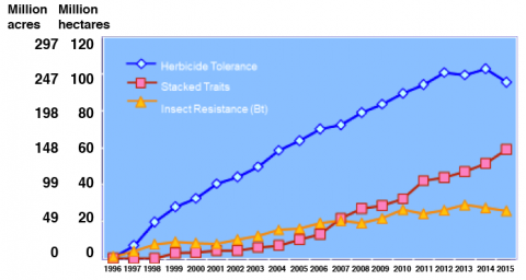
Not only have GM traits been rapidly adopted as VATs, the proportion of cultivars with combined, or stacked,GM traits has escalated quickly. Crops containing more than one GM trait were grown on nearly 60 million hectares globally in 2015 (Fig. 9).
SmartStax® Example
Not only do the stacks represent multiple value-added characteristics, some represent multiple genes (or events) for the same characteristic.
Let’s look at an example that demonstrates both scenarios: SmartStax® corn.
SmartStax® contains 8 genes conferring VATs:
- 3 genes for above-ground insect resistance to Lepidopteran species
- 3 genes for below-ground insect resistance to Corn Rootworm
- 2 genes for herbicide tolerance: one conferring tolerance to glyphosate herbicide and one conferring tolerance to glufosinate herbicide.
Thus, there are 4 VATs present in SmartStax®.
The sets of multiple genes for above- and below-ground insect resistance make it difficult for the insect species to overcome, whereas single genes are relatively easily overcome when enough selection pressure is applied. This pyramiding of genes conferring a given trait is a “best practice” as it is a key strategy for managing the development of resistance in pests and prolonging the utility of an architected solution (Fig. 10).
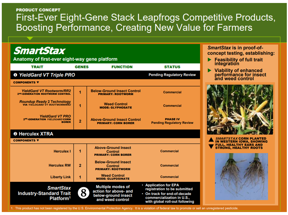
Also note that there are four events involved in delivering the 8 genes: MON88017, MON89034, TC6275, and DAS59122-7 for this product. Each event includes more than one gene, a condition referred to as “molecular stacking”.
GM Events Require Governmental Approvals
VATs created through genetic engineering are subject to government regulation on a country-by-country basis. Before approving cultivation or import of GM crops, governmental bodies generally review the issues related to:
- Problem addressed and effectiveness of the proposed solution.
- Food safety.
- Safety to the environment and biosphere.
The adoption of transgenic VATs in some countries is hampered by the lack of appropriate governmental bodies to review and authorize use.
Breeding strategies and transport of seed must take account of government regulations and comply with containment policies.
VATs Based on Gene Editing
Gene editing (or genome editing) comprises a range of molecular techniques that facilitate targeted changes to be made in the genome. It involves the use of certain nucleases to make precise cuts in the DNA, which then can become the sites of base pair substitutions, DNA deletions or DNA insertions, harnessing the organism’s own DNA repair system. Gene-editing techniques are typically named for the type of nuclease used.
For example, CRISPR-Cas9 involves:
- Clustered
- Regularly
- Interspaced
- Short
- Palindromic
- Repeats
coupled with a programmable nuclease derived from bacteria (Cas9).
For more details on genome editing, see the following YouTube videos:
Examples of VATs Created Through Gene Editing
Examples of VATs created through gene editing include:
SU CanolaTM – was developed by Cibus to provide a non-transgenic option to canola growers for weed control by conferring tolerance to sulfonylurea herbicides and is promoted for use with Draft™ herbicide from Rotam.
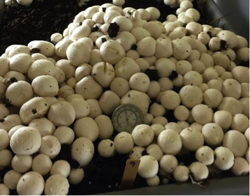
Non-browning mushrooms – were developed by Professor Yinong Yang at Pennsylvania State University using the CRISPR-Cas9 system. Several genomic deletions facilitated through gene editing have resulted in a product with longer shelf life and less post-harvest loss (Fig. 11). Commercialization is anticipated in the near future.
Maximizing the Use of VATs
You may have noticed the VATs that have been commercialized are branded (tradename, logo, etc.) to drive customer/consumer recognition and loyalty. Because VATs are in high demand and often have been developed at substantial investment, there is a desire to make the most of their use. From a breeding standpoint, this typically involves integrating each VAT into a wide array of elite cultivars to maximize market penetration.
Note that although stacking has been illustrated herein using a GM trait example, any type of VATs may be pyramided in a cultivar. Mixtures of types of combined VATs are not uncommon; many times the same customer/consumer base demanding one type of VAT may also demand others for maximum value.
Next, we will discuss ways to facilitate Trait Integration of single or multiple VATs through breeding.
Trait Integration
How does Trait Integration fit into an overall breeding program?
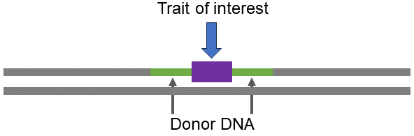
New elite lines produced through New Line Development and New Line Evaluation are converted for the VAT of interest through backcross breeding.
Elite Cultivar ➡ backcross breeding ➡ Elite Value-added Trait Cultivar
As a result, the breeder aims to recover the complete and unaltered agronomic package represented by the elite line plus the desired expression of all the genes or events introduced in the elite VAT cultivar.
Backcross Conversion Example
The general formula for integrating a single genetic factor (e.g., gene) via backcross (BC) conversion requires a cross between the trait donor (non-recurrent parent, NRP) and the elite line to be converted (recurrent parent, RP). Ideally, in each generation, only those individuals who inherit the desired gene are used as parents to create the next generation. Several generations of backcrossing to the RP are needed to recover the vast majority of the RP germplasm.
Once this is accomplished, individuals in the final backcross generation are self-pollinated to “fix” the introgressed gene in homozygous state. Progeny testing may be performed to identify non-segregating lines to bulk and label as the converted cultivar. In all, 11 or more generations may be required to complete the introgression of the desired gene (Table 1).
According to genetic theory, after six backcrosses the progeny are, on average, greater than 99% genetically similar to the RP.
| Generation | Plant | Activity | Produce |
|---|---|---|---|
| 1 | NRP, RP | Cross NRP to RP | F1 |
| 2 | F1 | Select for desired gene; BC to RP | BC1 |
| 3 | BC1 | Select for desired gene; BC to RP | BC2 |
| 4 | BC2 | Select for desired gene; BC to RP | BC3 |
| 5 | BC3 | Select for desired gene; BC to RP | BC4 |
| 6 | BC4 | Select for desired gene; BC to RP | BC5 |
| 7 | BC5 | Select for desired gene; BC to RP | BC6 |
| 8 | BC6 | Self | BC6S1 |
| 9 | BC6S1 | Self | BC6S2 |
| 10 | BC6S2 | Identify line phenotypically similar to RP that stably expresses introduced trait |
BC6S3 |
| 11 | BC6S3, tester | Create seed for testing performance equivalency; testcross (if RP is a hybrid parent) and/or self |
BC6S3 TC
BC6S4 |
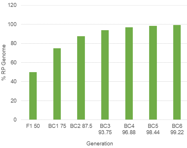
Recovery of RP Germplasm
Genetic theory indicates with each cross to the RP, the average percentage of NRP germplasm is reduced by half, assuming no selection. The general formula for calculating the estimated mean percentage of RP germplasm among backcross progeny in a given generation is:
[latex]\%RP(n) = 1 - (\dfrac{1}{2})^{n+1}[/latex]
where:
%RP = percentage of recurrent parent germplasm recovered
n = backcross generation number
In the BC6 generation, progeny on average are 99.22% genetically similar to the RP (Fig. 12).
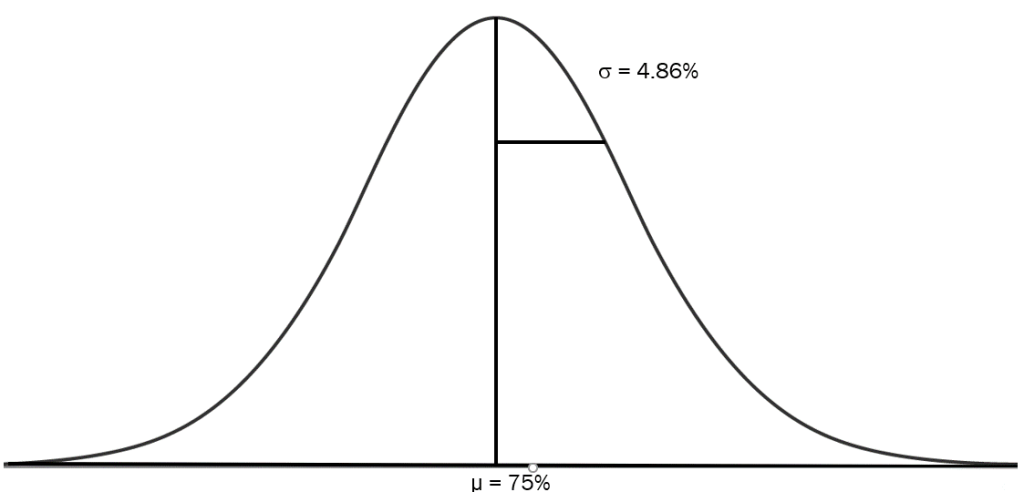
Backcross Population Distribution of %RP
However, all individuals in a given backcross generation do not contain the same proportion of RP germplasm. Each backcross generation represents a distribution of the percentage of RP germplasm. For example, the BC1 generation percentage of RP germplasm is normally distributed with a mean of 75% and a standard deviation of 4.86% (Fig. 13).
Distribution of Residual NRP Germplasm
However, in practice, with selection for the desired gene, more NRP germplasm remains and its distribution across the genome is not uniform.
Based on a 1788 centimorgan (cM) map of maize spanning 10 chromosomes, the mean amount of residual NRP germplasm was estimated using computer simulation (Peng et al. 2014). Note that the relationship between cM NRP and %RP is given by:
[latex]\%\textrm{RP}= \bigg[1-\dfrac{1}{2}\bigg(\dfrac{\text{cM NRP}}{\text{total NRP}} \bigg) \bigg] \times 100[/latex]
Thus, 120 cM of NRP germplasm in a genome of 1788 cM equates to approximately 96.6% RP.
For each BC generation, 1000 progeny were screened to identify those with the introgressed gene, with approximately half selected (single gene, Mendelian segregation). The mean NRP germplasm was estimated with these 500 individuals. In backcross generations BC1 through BC6, the mean residual NRP germplasm (in cM) was measured across the whole genome, on chromosomes not carrying the desired gene, on the chromosome carrying the desired gene, and in the region comprising 10 cM to each side of the desired gene (20 cM flanking region).
Although NRP germplasm on non-carrier chromosomes decreases incrementally with each backcross generation, the residual NRP germplasm on the carrier chromosome decreases at a much less rapid rate. Furthermore, the amount of residual NRP germplasm in the flanking region remains somewhat stagnant through 6 backcrosses; selection for the desired gene is pulling along linked DNA from the donor parent (Table 2).
| Total Genome NRP (cM) |
Non-Carrier
Chromosomes NRP (cM) |
Carrier
Chromosome NRP (cM) |
Flanking Region on the
Carrier Chromosome NRP (cM) |
n/a |
|---|---|---|---|---|
| BC1 | 1398.79 | 1240.62 | 158.17 | 19.53 |
| BC2 | 973.90 | 846.89 | 127.01 | 18.88 |
| BC3 | 681.45 | 578.13 | 103.32 | 18.26 |
| BC4 | 480.31 | 395.15 | 85.16 | 17.66 |
| BC5 | 343.20 | 271.49 | 71.71 | 17.12 |
| BC6 | 248.19 | 187.23 | 60.96 | 16.58 |
Linkage Drag
DNA in the chromosomal regions flanking a VAT is under pressure when backcross progeny with the VAT are identified and selected; recombination is reduced due to linkage with the VAT. The residual NRP in the chromosomal proximity with the desired gene is referred to as linkage drag (Fig. 14).
The effect of this linked DNA depends on the genetic contents of these chromosomal segments. Linkage drag can potentially affect performance for key traits like yield and stress tolerance.
Why?
This NRP germplasm may contain deleterious genes, especially if the trait donor is non-elite. If the introgressed genetic factor is a result of genetic engineering, this DNA from the NRP may have mutated during tissue culture, causing what is referred to as somaclonal variation. In the case of hybrid cultivars, if the trait donor is from the heterotic group opposite the RP, this DNA may decrease potential heterosis in the converted hybrid.
Linkage drag has the potential to interfere with the recovery of the performance of the RP and the goal to recover the complete and unaltered agronomic package represented by the elite line targeted for conversion! The impact of linkage drag can be magnified with the accumulated effect of multiple introgressed genes.
How can linkage drag be eliminated?
Identifying Homozygotes for the Desired Gene
Finally, once backcrossing has attained the desired level of RP germplasm recovery, the expression of the desired gene is stabilized through self-pollination to achieve homozygosity.
Since S1 plants will be segregating for the desired gene, continued self-pollination may be required to produce materials for progeny testing.
Efficiency in Trait Integration
Since Trait Integration requires additional time beyond New Line Development and New Line Evaluation and additionally presents some risk in recovering the full set of performance attributes of the line targeted for conversion, there may be some opportunities to utilize technology in an efficient manner to reduce these negatives. Specifically, the application of technology to accelerate the conversion process and to reduce the risk of failure to recover performance equivalency to the RP would represent an enormous improvement in efficiency.
Strategically, technology addressing the following issues would make Trait Integration more efficient and effective, while increasing the rate of genetic gain:
- Selection accuracy
- Effective screen for desired gene/trait.
- Identification based on genotype (vs. phenotype).
- Acceleration of the process
- Faster cycling of generations.
- Quicker recovery of RP germplasm in backcrossing.
- Fewer generations for gene/trait fixation.
- Quality outcomes
- Eliminating linkage drag.
- Ensuring a high degree of recovery of %RP.
Use of Molecular Markers for Greater Efficiency in Trait Integration
Molecular markers are a great fit for technology to meet the need for selection accuracy, acceleration, and quality outcomes. Molecular markers provide knowledge of genotypes among backcross progeny. The use of this technology has great advantages over trait integration (TI) based on phenotype alone (Table 3).
| Molecular markers can be used to: | n/a | Conduct marker-assisted backcrossing (MABC) to: |
| Identify individuals that have inherited the desired gene | to | Be more efficient than phenotypic selection |
| Select for recovery of RP germplasm in backcross generation | to | Trim ≥3 generations from the TI process to save 1-2 years in the development of VAT hybrids |
| Select against linkage drag | to | Select against linkage drag to increase the probability of obtaining acceptable (i.e. quality) conversion |
| Identify homozygotes for the VAT gene(s) in the selfing generations | to | Reduce the number of generations to trait fixation |
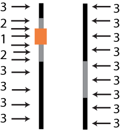
MABC Selection Schemes
With marker(s) for the desired gene, a set of markers that provides coverage of the genome, and a set of dense markers (one per cM in the 20 cM region flanking the desired gene), it is possible to implement (Fig. 15):
- Selection for the target gene/event (selection for those individuals that carry the desired genetic factor).
- Selection against linkage drag (selection for individuals with crossovers in the flanking region).
- Selection for RP recovery (selection for those individuals in the upper tail of the backcross population distribution).
Designing an Efficient Trait Integration Process
Although we have been discussing the principles of single gene integration, in real life the integration typically involves multiple VATs or multiple genetic factors. Thus, pyramiding of all the genetic factors involved is necessary.
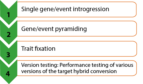
Multiple Trait Integration involves four steps (Fig. 16):
Computer simulation has value in designing a product pipeline to improve the process of Trait Integration, especially since there are a considerable number of options when converting a particular cultivar for multiple genetic factors. Computer simulation offers the opportunity to identify options that can garner efficiency in terms of speed to market, rate of gain, conservation of resources, etc.
An example of using computer simulation to drive a strategic approach for multiple Trait Integration is given through a study conducted in the Mumm Lab at the University of Illinois.
Efficiencies Revealed Through Computer Simulation
A study was conducted to explore the limits of Multiple Trait Integration and identify strategies that could result in recovery of equivalent performance in a corn hybrid converted for 15 events (Peng et. al. 2014a, 2014b; Sun and Mumm 2015). Conversion for 15 genetic factors was considered to be pushing the boundaries of what could be accomplished with backcross conversion since traditionally a limit of about 5 stacked genes was accepted practice.
The breeding scenario assumed:
- Some events were required in the male parent of the hybrid so a decision was made to balance the 15 events between the female and male RPs: 8 events would be introgressed into female RP and 7 events into male RP.
- All events are new so conversions for each event are needed.
- Residual NRP germplasm in the 20 cM region flanking the introgressed event (FR NRP) will be unalterable after Step 1 (once pyramiding is initiated).
- Population size of 400 each generation, with final selection of the top four plants (selected proportion = 0.01).
Since 120 cM of NRP germplasm (~ 6.7% NRP) is the maximal amount of residual NRP germplasm consistent with recapturing target hybrid performance, a goal for single event conversions was set at ≤8 cM Total NRP including ~1 cM of FR NRP.
Optimization Criteria
To identify optimal breeding strategies for Step 1 in the Multiple Trait Integration process with the aim to minimize accumulation of linkage drag in the converted target hybrid and maximize efficiencies, several criteria by which to assess efficiency were defined:
- Total NRP (cM).
- FR NRP (cM).
- Time (expressed in generations).
- Marker data points (MDP).
- Population size (N).
The greatest priority is given to Numbers 1 and 2 since these criteria determine the effectiveness of the integration process outcome, that is, the ability to recover equivalent performance. Without this, all resource expenditures and time investment in Trait Integration to further improve the elite hybrid is meaningless. Number 3 impacts genetic gain in a major way. And Numbers 4 and 5 determine resources in terms of budget, manpower, and facilities (e.g., genotyping costs, labor, greenhouse, field space).
Findings of Computer Simulation Study
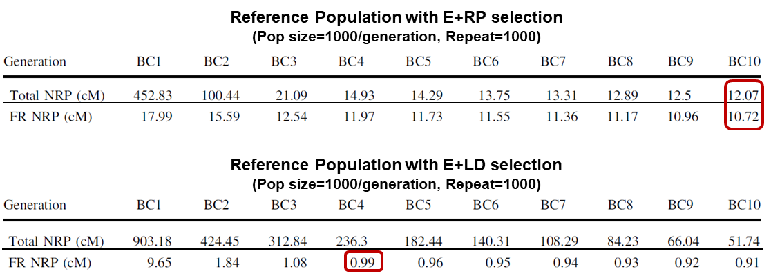
The goal of the computer study was to identify an optimal strategy for selection for the particular event (E), selection against linkage drag (LD), and selection for percent RP germplasm (RP).
Preliminary investigation showed, based on selection for E+RP, that Total NRP would be reduced to about 12 cM after 10 generations of backcrossing, yet most of the residual NRP germplasm would reside in the flanking region (FR).
On the other hand, if selection was based on E+LD, the Total NRP remained high but FR NRP was reduced to ~1 cM by BC3 or BC4 and remained largely static after that. It seemed highly unlikely that FR NRP would be reduced much beyond 1 cM, even with extensive additional backcrossing (Fig. 17).
Additional Simulation Results
All combinations of selection for E, LD, and RP were considered with the goal of reducing Total NRP to ≤8 cM and FR NRP to ~1 cM.
The objective was nearly met with 5 generations of selection, the first 3 generations for E+LD followed by 2 generations of E+RP. Total NRP was reduced to 7.86 cM. However, the FR NRP was at 1.68 cM — more work was needed (Table 4).
| Selection Methods |
MAS Gen. |
BC1 | BC2 | BC3 | BC4 | BC5 | Total Non-RP (cM) |
FR Non-RP (cM) |
MDP (K) |
Ntotal |
|---|---|---|---|---|---|---|---|---|---|---|
| Three-Stage | 5 MAS | E+LD+RP | E+LD+RP | E+LD+RP | E+LD+RP | E+LD+RP | 17.85 | 1.42 | 222 | 2000 |
| 4 MAS | E | E+LD+RP | E+LD+RP | E+LD+RP | E+LD+RP | 31.02 | 1.80 | 178 | 1608 | |
| 3 MAS | E | E | E+LD+RP | E+LD+RP | E+LD+RP | 47.70 | 2.67 | 134 | 1216 | |
| 2 MAS | E | E | E | E+LD+RP | E+LD+RP | 75.68 | 5.17 | 89 | 824 | |
| 1 MAS | E | E | E | E | E+LD+RP | 148.28 | 9.73 | 45 | 432 | |
| Two-Stage | 5 MAS | E+LD | E+RP | E+RP | E+RP | E+RP | 14.83 | 7.81 | 166 | 2000 |
| E+LD | E+LD | E+RP | E+RP | E+RP | 8.65 | 3.43 | 130 | 2000 | ||
| E+LD | E+LD | E+LD | E+RP | E+RP | 7.86 | 1.68 | 94 | 2000 | ||
| E+LD | E+LD | E+LD | E+LD | E+RP | 19.17 | 1.27 | 58 | 2000 | ||
| 4 MAS | E | E+LD | E+RP | E+RP | E+RP | 14.68 | 7.50 | 126 | 1608 | |
| E | E+LD | E+LD | E+RP | E+RP | 9.59 | 3.09 | 90 | 1608 | ||
| E | E+LD | E+LD | E+LD | E+RP | 21.86 | 1.69 | 54 | 1608 | ||
| 3 MAS | E | E | E+LD | E+RP | E+RP | 16.38 | 7.54 | 86 | 1216 | |
| E | E | E+LD | E+LD | E+RP | 21.47 | 3.13 | 50 | 1216 | ||
| 2 MAS | E | E | E | E+LD | E+RP | 39.27 | 7.94 | 45 | 824 | |
| Combined | 5 MAS | E+LD | E+LD+RP | E+LD+RP | E+LD+RP | E+LD+RP | 21.16 | 1.33 | 182 | 2000 |
| E+LD | E+LD | E+LD+RP | E+LD+RP | E+LD+RP | 30.99 | 1.26 | 142 | 2000 | ||
| E+LD | E+LD | E+LD | E+LD+RP | E+LD+RP | 54.87 | 1.19 | 102 | 2000 | ||
| E+LD | E+LD | E+LD | E+LD | E+LD+RP | 108.24 | 1.15 | 62 | 2000 | ||
| 4 MAS | E | E+LD | E+LD+RP | E+LD+RP | E+LD+RP | 40.53 | 1.61 | 138 | 1608 | |
| E | E+LD | E+LD | E+LD+RP | E+LD+RP | 64.04 | 1.49 | 98 | 1608 | ||
| E | E+LD | E+LD | E+LD | E+LD+RP | 117.18 | 1.38 | 58 | 1608 | ||
| 3 MAS | E | E | E+LD | E+LD+RP | E+LD+RP | 69.41 | 2.25 | 94 | 1216 | |
| E | E | E+LD | E+LD | E+LD+RP | 117.05 | 1.94 | 54 | 1216 | ||
| 2 MAS | E | E | E | E+LD | E+LD+RP | 113.32 | 4.63 | 49 | 824 |
Refining the Strategy
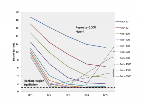
To fine-tune the strategy, population size was considered as a possible means to reducing FR NRP. By increasing population size during the generations involving E+LD while continuing the same selection intensity, the probability of recovering some individuals with less FR NRP is increased (Fig. 18). Recall that equilibrium for FR NRP is reached when residual NRP in the region is about 1 cM.
Optimizing the Strategy
To build on the earlier simulation results, strategies with varied population sizes for the three generations of E+LD selection were considered. In conclusion, Peng et. al. (2014a) found that the strategy involving five generations of selection, the first three generations for E+LD with a population size of 600 followed by two generations of selection for E+RP with a population size of 400, resulted in 6.57 cM of Total NRP with 1.18 cM in the flanking region. Goal achieved!
This strategy required 100,600 marker data points and 2600 individual backcross progeny overall (Table 5). Costs for these could be estimated to provide a comprehensive view of the budget implications versus benefits of implementing this strategy in Trait Integration.
| Strategy | BC1 E+LD |
BC2 E+LD |
BC3 E+LD |
BC4 E+RP |
BC5 E+RP |
Total NRP |
FR NRP |
MDP (K) |
Ntotal |
|---|---|---|---|---|---|---|---|---|---|
| 1 | 400 | 400 | 400 | 400 | 400 | 7.86 | 1.68 | 94.0 | 2000 |
| 2 | 600 | 600 | 600 | 400 | 400 | 6.57 | 1.18 | 100.6 | 2600 |
| 3 | 800 | 800 | 800 | 400 | 400 | 6.10 | 1.13 | 107.2 | 3200 |
Choosing Future Donor Parents
Of course, once “clean” conversions have been achieved, these can be used as trait donors in subsequent conversions. With only ~1 cM of non-elite DNA surrounding the event of interest (genetic factor), such conversions represent an excellent choice as donor parent to initiate new VAT conversions.
What other factors should be considered in choosing the donor parent for VAT conversions?
Genetic similarity to the line targeted for conversion would be beneficial since the goal of backcrossing is to recover the likeness of the RP. If the donor parent is related to the RP, then fewer backcross generations would be required to recover the RP attributes.
Computer simulation showed that if the NRP is 30% similar genetically to the RP, then complete conversion can be achieved by BC4 using markers for selection of E, LD, and RP. If the NRP is 86% similar genetically to the RP, then complete conversion can be achieved by BC3.
Refer to Molecular Plant Breeding for more details.
Next Steps
The results for Single Gene/Event Introgression indicated that the goal of a very “clean” conversion was achievable!
Furthermore, it sets the stage for optimizing the other steps in Multiple Trait Integration: Gene/event Pyramiding, Trait Fixation, and Version Testing (Fig. 17).
More on the Simulation Scenario
Continuing further with the breeding scenario to convert a corn hybrid for 15 events, some additional assumptions were added as next steps in Multiple Trait Integration were analyzed:
- Hybrid conversions involved stacking 8 events in the female parent RPF of the hybrid
and 7 events in the male parent RPM of the hybrid. - On each side of the pedigree, events are on different chromosomes (unlinked).
- Up to 5 versions of each converted hybrid were considered.
- The target hybrid yielded 14.72 tons per hectare (i.e. 235.6 bushels per acre) on average.
- The overarching objective is recovery of a converted hybrid that yields within 3% of the target hybrid.
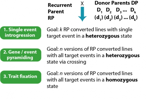
The goals for each step are defined by the desired outcome. For example, the outcome of Single Event Introgression is k versions of each RP, each of the k versions representing a single event introgression into the RP background, created through backcrossing. With 8 events being stacked in the female parent of the hybrid, k = 8 for RPF. At the close of Single Event Introgression, the backcross lines carry the desired event in a heterozygous state (Fig. 19).
Event Pyramiding
Once quality single-event RP conversions have been created, the most efficient way to combine the events in the RP background is with a set of symmetrical crosses.
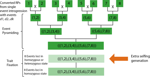
To stack 8 events in the RPF: first, pairs of single event lines are crossed, then the double-event progeny are crossed, and finally the quad-event progeny are crossed to combine all 8 events in the RPF background. Thus, 3 generations are required to combine all 8 events in heterozygous state in the specific RP.
Note that, although the simulation considered all events for a particular RP unlinked, in real life, linked events demand special attention in crossing to minimize the occurrence of repulsion linkages.
Trait Fixation
Theoretically, it would take a single generation of self-pollination to recover at least one progeny that is homozygous for all 8 events; each single event would be segregating in Mendelian fashion. However, the probability of recovering such an individual is very small.
Therefore, an extra generation may be introduced to alleviate bottlenecking due to extremely low frequency of the desired genotype. This concept is referred to as “F2 enrichment” as per Bonnett et al. (2005). The outcome of the extra generation of self-pollination is it allows for individuals that have at least one copy of every event to be advanced (Fig. 20).
Practical Considerations
Two factors are very important to determining success in recovering specific desired genotypes: the population size and the expected frequency of the desired genotype in the population. Another factor is the number of individuals to be recovered. These factors must be stated for each generation.
The expected frequency of the desired genotype is a probability function based on Mendelian genetics. Note the example below (Table 6).
| Generation | Pyramid 2 Events | Pyramid 4 Events | Pyramid 8 Events | S1 with 8 Events in heterozygous/ homozygous state |
S2 with 8 Events in homozygous state |
|---|---|---|---|---|---|
| Genotype/Event | Aa | Aa | Aa | AA/Aa | AA |
| Formula | (0.5)2 | (0.5)4 | (0.5)8 | (0.75)8 | (0.5)8 |
| Probability | 0.25 | 0.0625 | 0.00390625 | 0.100112915 | 0.00390625 |
Determining Minimum Population Size
Knowing the expected frequency of the desired genotype and stipulating the number of individuals to be recovered as well as the probability of success, the necessary minimum population size can be determined.
Based on the binomial distribution (Sedcole 1977):
[latex]\sum_{i=x}^{N}\binom{N}{i}p^{i}(1-p)^{N-i} ≥ q[/latex]
where:
N refers to the minimal population size
x is the number of recovered individuals with the desired genotype
p is the probability of achieving the breeding goal
q is the frequency of the desired genotype in the population.
For the special case of x=1, the following formula applies:
[latex]N\geq ln(1-p)/ln(1-q)[/latex]
To recover with 99% probability at least one plant with a genotype expected at the 0.25 frequency in the population,
[latex]N\geq ln(1-.99)/ln(1-.25)[/latex]
[latex]N\geq16.00784556[/latex]
Thus, 99% of the time, 17 plants are needed to recover ≥1 with the desired genotype when that genotype is expected to occur in 1 in 4 individuals in the population.
Population Size Guide
Sedcole (1977) provided a handy table to help in quickly estimating the population size needed to guarantee recovery of desired genotypes with high probability (Table 7).
| p* | q^ | 1 | 2 | 3 | 4 | 5 | 6 | 8 | 10 | 15 |
| 0.95 | 1/2 | 5 | 8 | 11 | 13 | 16 | 18 | 23 | 28 | 40 |
| 1/3 | 8 | 13 | 17 | 21 | 25 | 29 | 37 | 44 | 62 | n/a |
| 1/4 | 11 | 18 | 23 | 29 | 34 | 40 | 50 | 60 | 84 | n/a |
| 1/8 | 23 | 37 | 49 | 60 | 71 | 82 | 103 | 123 | 172 | n/a |
| 1/16 | 47 | 75 | 99 | 122 | 144 | 166 | 208 | 248 | 347 | n/a |
| 1/32 | 95 | 150 | 200 | 246 | 291 | 334 | 418 | 500 | 697 | n/a |
| 1/64 | 191 | 302 | 401 | 494 | 584 | 671 | 839 | 1002 | 1397 | n/a |
| 0.99 | 1/2 | 7 | 11 | 14 | 17 | 19 | 22 | 27 | 32 | 45 |
| 1/3 | 12 | 17 | 22 | 27 | 31 | 35 | 44 | 52 | 71 | n/a |
| 1/4 | 17 | 24 | 31 | 37 | 43 | 49 | 60 | 70 | 96 | n/a |
| 1/8 | 35 | 51 | 64 | 77 | 89 | 101 | 124 | 146 | 198 | n/a |
| 1/16 | 72 | 104 | 132 | 158 | 182 | 206 | 252 | 296 | 402 | n/a |
| 1/32 | 146 | 210 | 266 | 218 | 268 | 416 | 508 | 597 | 809 | n/a |
| 1/64 | 293 | 423 | 535 | 640 | 739 | 835 | 1020 | 1198 | 1623 | n/a |
| * = probability of recovering r plants with trait. ^ = probability of occurrence of trait. |
||||||||||
Further Efficiencies in Trait Fixation
Further efficiency in Trait Fixation can be considered in terms of plant materials for genotyping (e.g. seed chipping before planting or sampling leaf tissue of seedling plants). Bottom line: with seed chipping, selection can be performed before planting so resources are focused only on the individuals with the desired genotype.
In addition, cycle time is decreased because the S2 outcome of selection is determined before planting. If testcrossing is required to facilitate version testing, the S2 materials can be planted appropriately to produce the hybrids.
Trait Fixation also results in the production of Breeder Seed to hand-off to Supply Chain. Those individuals deemed to be fixed for the introgressed genetic factors will be self-pollinated to produce seed which can be bulked to comprise the converted new elite line. The hand-off to Supply Chain will occur once the performance equivalency of the converted line has been confirmed.
Further Efficiencies Overall Through Rapid Cycling
In addition to accomplishing the breeding goal each generation, the entire process of Trait Integration can be accelerated through rapid cycling of the generations for backcrossing, pyramiding, and trait fixation. In other words, ways to achieve more than one generation per year speed the process.
This can be accomplished through the use of off-season nurseries, continuous nurseries in tropical locations, or the greenhouse to facilitate the continual rapid cycling of generations. With corn, continuous nurseries have enabled the cycling of four generations per year. Methods of intensive nursery management resulting in a rapid progression of generations have been referred to as speed breeding.
Version Testing
For the final step in Multiple Trait Integration, the converted cultivar is tested to assess its performance against its unconverted counterpart. The goal is performance equivalency.
The factors that determine success are:
- The amount of residual NRP germplasm in the converted cultivar.
- The probability of successful recovery of at least one version of the cultivar with equivalent performance.
- The number of stacked versions of each RP.
Just because the conversions have been created, it does not mean that performance equivalency has been recaptured. However, Sun and Mumm (2015) showed that, given the strict standards of single event conversions shown, there is a high likelihood of recovering an equivalent conversion even when the conversion involves 15 stacked events. Encouraging!
See Sun and Mumm (2015) for more details.
This chapter has focused on the Trait Integration component of the product pipeline, an important element in cultivar development. In addition, it has featured results of a study in process design for Trait Integration, because efficiency that leads to a higher rate of genetic gain is a critical part of getting better cultivars into farmers’ hands.
The next chapter will consider ways to further optimize the product pipeline.
References
Bonnett, D.G., G.J. Rebetzke, W. Spielmeyer. 2005. Strategies for efficient implementation of molecular markers in wheat breeding. Molecular Breeding. 15:75-85.
Comai, L., S. Henikoff. 2006. TILLING: Practical single-nucleotide mutation discovery. Plant J. 45:684-694. DOI: 10.1111/j.1365-313X.2006.02670.x
Fehr, W. R. 1987. Principles of Cultivar Development Volume 1: Theory and Technique. McMillan Publishing Company.
Ishii, T., and K. Yonezawa. 2007a. Optimization of the Marker-Based Procedures for Pyramiding Genes from Multiple Donor Lines: I. Schedule of crossing between the donor lines. Crop Sci. 47(2):537-546.
Ishii, T., and K. Yonezawa. 2007news.psu.edu/…/gene-edited-mushroom-created-penn-state-researcher-changing-gmob. Optimization of the Marker-Based Procedures for Pyramiding Genes from Multiple Donor Lines: II. Strategies for selecting the objective homozygous plant. Crop Sci. 47:1878-1886.
James, Clive. 2015. 20th Anniversary (1996 to 2015) of the Global Commercialization of Biotech Crops and Biotech Crop Highlights in 2015. ISAAA Brief No. 51. ISAAA: Ithaca, NY.
Monsanto-DowAgrosciences Collaborative Agreement Presentation, September 14, 2014.
Mumm, R.H. 2013. A look at seed product development with genetically modified crops: Examples from maize. J. Agri. and Food Chem. 61(35):8254-8259. DOI: 10.1021/ jf400685y
Peng, T., X. Sun, and R.H. Mumm. 2014a. Optimized breeding strategies for multiple trait integration: I. Minimizing linkage drag in single event introgression. Molecular Breeding 33:89-104. DOI 10.1007/s11032-013-9936-7
Peng, T., X. Sun, and R.H. Mumm. 2014b. Optimized breeding strategies for multiple trait integration: II. Process efficiency in event pyramiding and trait fixation. Molecular Breeding 33:105-115. DOI 10.1007/s11032-013-9937-6
Sun, X., T. Peng, and R.H. Mumm. 2011. The role and basics of computer simulation in support of critical decisions in plant breeding. Molecular Breeding 28 (4):421-436. http://www.springerlink.com/openurl.asp?genre=article&id= doi:10.1007/s11032-011-9630-6
Sun, X., and R.H. Mumm. 2015. Optimized breeding strategies for multiple trait integration: III. Parameters for success in version testing. Molecular Breeding 35:201. DOI 10.1007/s11032-015-0397-z
Till, B.J., S.H. Reynolds, C. Weil, N. Springer, C. Burtner, K. Young, E. Bowers, C.A. Codomo, L.C. Enns, A. R. Odden, E. A. Greene, L. Comai, S. Henikoff. 2004. Discovery of induced point mutations in maize genes by TILLING. BMC Plant Biology 4:12. DOI:10.1186/1471-2229-4-12
How to cite this chapter: Mumm, R.H. (2023). Value-added Trait Integration. In W. P. Suza, & K. R. Lamkey (Eds.), Cultivar Development. Iowa State University Digital Press.
Mutagenesis is a process by which the DNA of an organism is changed, resulting in a mutation. It may occur spontaneously in nature, in response to exposure to mutagens. Mutagenesis can also be initiated intentionally through guided laboratory procedures exposing plant materials to mutagens.
Quantitative Trait Locus/Loci
M1 is the first generation after mutagenesis.
M2 is the second generation after mutagenesis.
Interruption of the transcription or translation of DNA such that a gene is not expressed phenotypically.
Multiple traits pyramided into a single cultivar.
A converted line represents an isogenic or near isogenic change affected through backcross breeding.
refers generally to a gene, event, QTL, or other DNA segment.
Fixation represents the absence of segregation because all alleles at a particular locus are the same.
