
Human Nerve Conduction Velocity (NCV)
The NCV Test
Karri Haen Whitmer
Background
Conduction of an impulse in human nerves relies upon the electrochemical activity of the individual neuron fibers inside the nerve. Each fiber (axon) inside the nerve is capable of propagating an action potential if the stimulus is strong enough to bring the membrane potential of the neuron to the threshold value. Depending on the strength of the stimulus, not all fibers in a nerve may fire. Despite this, the action potential is an all-or-none phenomenon, where it will always have the same amplitude and time course for a single neuron. When action potentials are recorded via recording electrodes on the skin, the result is a “compound action potential,” which is an algebraic sum of action potentials from many cells. We have already observed compound muscle action potentials (CMAP) in the EMGs of previous labs.
Signal transmission within and between neurons
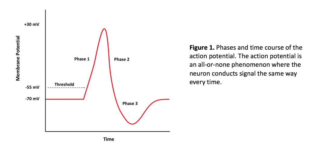
The action potential is the converse of the cell membrane resting potential, which, for neurons registers -70 mV on the voltmeter. The action potential involves several steps, starting with the onset of a stimulus. Most of the time, stimuli generating action potentials are chemical, where a ligand, a neurotransmitter, binds to a ligand-gated ion channel in the cell membrane of the dendrite or cell body of the neuron. If the graded potential is excitatory and sufficiently strong, the dissipation of charge across the cell body membrane reaches the axon hillock and depolarizes the cell membrane to -55 mV. The axon hillock is a region of high voltage-gated ion channel density.
Voltage gated channels open in response to threshold depolarization of the membrane, leading to an influx of sodium (via the voltage gated sodium channel), bringing about the onset of Phase 1 of the action potential (Figure 1). The influx of sodium drives the membrane potential to +30 mV, which is the peak of the action potential on a graph. From here, voltage gated potassium channels, which slowly open near the end of Phase 1 of the action potential, allow efflux of potassium from the cell. The membrane repolarizes in response to the efflux of potassium, and the membrane potential reaches resting potential at the end of Phase 2. However, because the potassium channels close very slowly compared to sodium channels, the continued leakage of potassium from the cell results in membrane hyperpolarization, during which the membrane potential reaches -90 mV. At the end of phase 3, the activity of the sodium/potassium ATPase active transporter, which exports three sodium ions and imports two potassium ions helps to bring the membrane potential back to -70 mV (along with passive sodium and potassium leak channels).
In order to communicate the signal of the action potential to another cell, synaptic transmission must occur. Synaptic transmission is the rate-limiting step of neural transmission, meaning that it is the slowest part of signal transmission. During synaptic transmission, the action potential reaches the axon termini of the pre-synaptic cell. The influx of sodium depolarizes the membrane of the termini and opens voltage gated calcium channels. Calcium enters the cell, resulting in the fusion of neurotransmitter-filled vesicles with the pre-synaptic membrane.
Neurotransmitter diffuses across the synaptic cleft and binds to a receptor on the post-synaptic cell. The binding of neurotransmitter to a receptor will cause a post-synaptic potential (PSP) (a graded potential). Post-synaptic potentials may be excitatory or inhibitory, depending on the interaction of the neurotransmitter with the receptor.
Speed of neural transmission
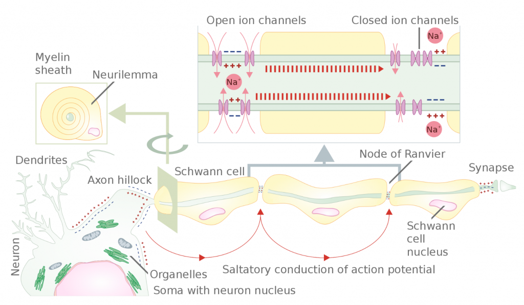
The speed of neuron transmission generally depends upon two factors: axon size and degree of myelination. Larger diameter axons transmit signal faster due to lower resistance to the flow of charge inside the axon. Myelinated axons (white matter) transmit action potentials faster, up to approximately 150 m/s, due to saltatory conduction (Figure 2). In saltatory conduction, ion channels are only necessary between regions of myelination (Nodes of Ranvier); thus, the signal dissipates quickly under regions of myelination to each node and is re-established there, until the signal reaches the terminus. On the other hand, in unmyelinated axons (gray matter), conduction is continuous. This means signal transmission is relatively slow because the voltage gated ion pumps must be present, and used, on all regions of the axonal membrane. Continuous conduction speeds rarely reach 10 m/s. Nerve conduction velocities, which are calculated as the result of the transmission of hundreds or thousands of action potentials firing along the axons of neurons inside nerves, may be affected by the health of the nervous system, age, sex, and even temperature.
Disease and neural transmission
Electromyograms (EMGs) are a non-invasive way to determine nerve conduction velocities in the clinical setting. In one type of nerve conduction velocity test (NCV) an EMG recording electrode detects the contraction of a muscle in response to direct neural stimulation by a stimulating electrode placed upon the skin. The time from the onset of stimulus (firing of the stimulating electrode) until muscle contraction is recorded. The stimulating electrode is then moved and the measurement is taken again. From this information, one can determine the nerve conduction velocity.
Nerve conduction velocities inform us about the relative health of peripheral nerves. Damage to nerves or diseases that cause demyelination (such as multiple sclerosis – MS) or nerve degeneration (like amyotropic lateral sclerosis – ALS) are primary concerns when conduction speeds are undetectable or below the normal range. The peripheral nerves of the arms generally have conduction velocities between 50-60 m/s.
Interpreting EMGs resulting from direct electrical stimulation of a nerve
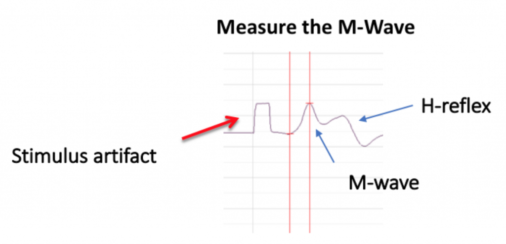
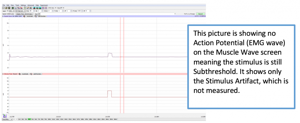
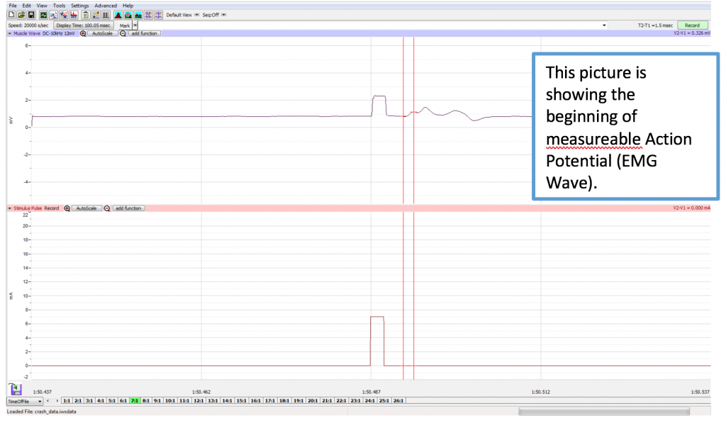
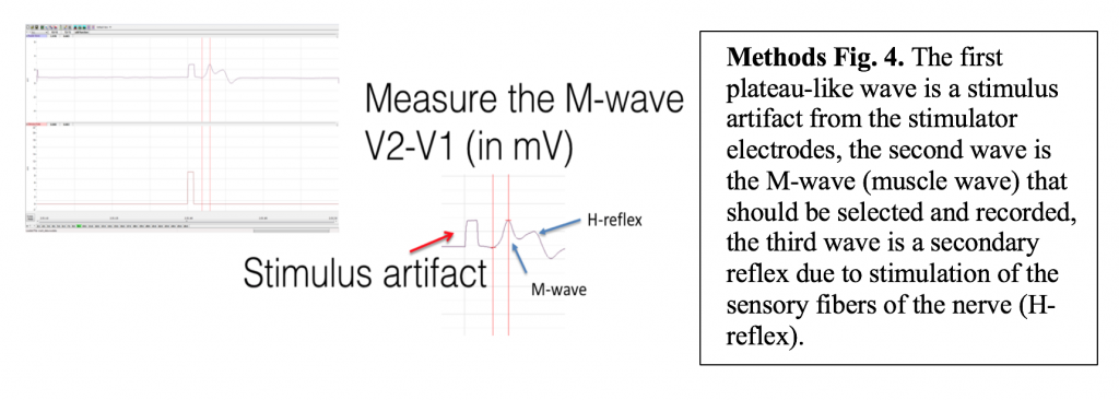
Because there are both sensory and motor fibers in the Ulnar nerve, both will be stimulated upon application of stimulating electrodes to the skin. Activation of sensory fibers will initiate the “H-reflex,” for which the pathway includes the sensory neurons, integrating center (spinal cord), and motor neurons. This is much like we saw last week in the muscle spindle reflex experiments. Application of current to the ulnar nerve also results in an M-wave, an EMG wave due to direct activation of the motor neurons, which will quickly produce a muscle response. In this lab, we will take measurements from the M-waves, only. Note that passive transmission of current in body tissues from the stimulating electodes also produces a stimulus artifact on the EMG. Please see the figure below (Figure 3).
This week’s experiment:
This week, we will perform one experiment (lab exercise 1) and one clinical evaluation (lab exercise 2). The experiment will determine the effects of increasing stimulus strength on the EMG. Stimulus (measured in milliamperes, mA) is applied directly to the fibers of the ulnar nerve with stimulating electrodes on the skin. The resulting EMG amplitude is recorded in mV. EMG amplitude measures the strength of contraction by the innervated muscle, which is relative to the number of motor units activated by the stimulus. Recruitment of more motor units (activation of additional motor neurons and their innervated muscle cells) is accomplished by increasing the stimulus.
Next, we will perform a nerve conduction study using EMG. Here, we will use the optimal stimulus strength from Experiment 1 to re-stimulate the ulnar nerve. After recording the location of the stimulating electrode on the arm and obtaining the EMG, the stimulator will be moved to a secondary position, re-stimulating the ulnar nerve. Here, we will divide the physical distance between the stimulators (in mm) by the difference in time between the two trials’ M-waves on the EMG. This method of calculating conduction velocity is called the difference method.
Measurements in this lab:
In this week’s lab, we will measure the effect of stimulus strength on the amplitude of the compound muscle action potential visualized on the electromyogram. We will then use the information from our experiment to determine the conduction velocity (transmission speed) of the ulnar nerve in a nerve conduction study.
To help prepare for this week’s lab, answer the following:
- What is the dependent variable tested in this week’s experiment (lab exercise 1)?
- What independent variable is tested in this week’s experiment (lab exercise 1)?
- Can you think of an experiment you could conduct using the methods of the nerve conduction study (lab exercise 2)? Hint: what kinds of variables might affect the speed of nerve transmission?
Laboratory Methods for iWorx
Laboratory Methods Highlights
· This week, instead of stimulating a nerve with a reflex hammer via stretch receptors, we will stimulate a nerve directly with stimulating electrodes.
· Please wear short sleeves or sleeves that can be rolled above the elbow, half way up the brachium.
· A stimulating electrode delivers a mild electric shock, which, if sufficiently strong, depolarizes the membranes of neurons, causing them to fire.
· Neurons stimulated with stimulating electrodes behave like other neurons, except that when stimulating the fibers of a nerve, we may provoke action potentials in both sensory and motor fibers at the same time.
· In this lab we will stimulate the ulnar nerve and determine the outcome of increasing stimulus strength (in mAmps).
· Later, we will re-stimulate the ulnar nerve from two different locations along the arm in order to determine the conduction velocity.
Equipment Required: IXTA data acquisition unit, iWire-B3G cable and three EMG lead wires, disposable snap electrodes, HV stimulator lead wires.
I. Equipment Setup: Start the Software
Turn on the iWorx hardware box at the switch on the back, and select the Week7_NerveConduction.iwxset file from the P-drive.
II. Equipment Setup: Electrode Placement
- The subject should remove all jewelry from his/her left or right hand and wrist.
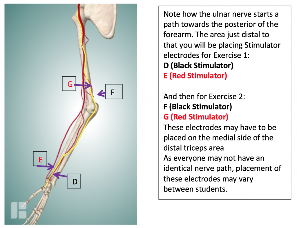
- Study the pathway of the ulnar nerve in the picture (below).
3. Clean the areas where the electrodes will be attached with an alcohol pad. Lightly abrade the skin in those areas.
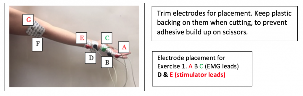
- Obtain Seven disposable electrodes. Label 5 them on the pointed tab with the letters A through E.
- Cut down the electrodes so just the Medline logo shows. Keep the plastic backing on them to reduce adhesive build up on the scissors.
- Place A on the medial edge of the little finger of the right hand, so the electrode button/snap is just above the first knuckle. This is for the RED (+) recording electrode in Figure HN-3-S2.
- Place B on the medial edge of the palm, so the electrode button/snap is at the base of the little finger. This is for the BLACK (-) recording electrode on the hand.
- Place C so the electrode button/snap is on the medial edge of the wrist just above the crease of the wrist. This is for the GREEN ground electrode on the hand.
- Warning: Before connecting the IXTA stimulating electrodes to the subject, check the Stimulator Control Panel in the LabScribe toolbar to make sure the amplitude value is set to zero (0 AMP).
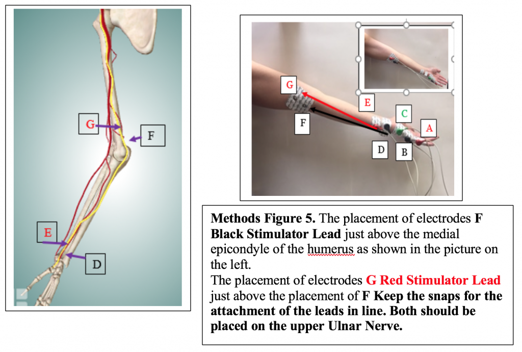
Next, attach the remaining 2 electrodes to the subject’s arm so that they are placed on the pathway of the Ulnar Nerve in the following configuration:
- Place D the medial edge of the forearm, so the electrode button/snap is above the wrist crease. Attach the BLACK (-) stimulating electrode.
- Place E, the positive stimulating electrode, right above the negative stimulating electrode towards the medial side of the forearm. Attach the RED (+) stimulating electrode.
- Electrodes F and G (in the photo) will be placed later for Exercise 2.
- Videos of proper electrode placement for Exercises 1 and 2 are found on the P-Drive.
Safety precautions for this lab:
You will deliver mild electric shocks to either yourself or a volunteer experimental subject. The equipment you use to do this is carefully designed to keep the parameters of the electroshocks well within a safe range, and this experiment is safe and fun. Nevertheless, we ask that you place stimulating electrodes on the arms only, and only place electrodes on the same side of the body (never on both arms at the same time).
If you think you may be pregnant or if you suffer from known heart conditions or have an artificial heart pacemaker please do not volunteer as an experimental subject this week.
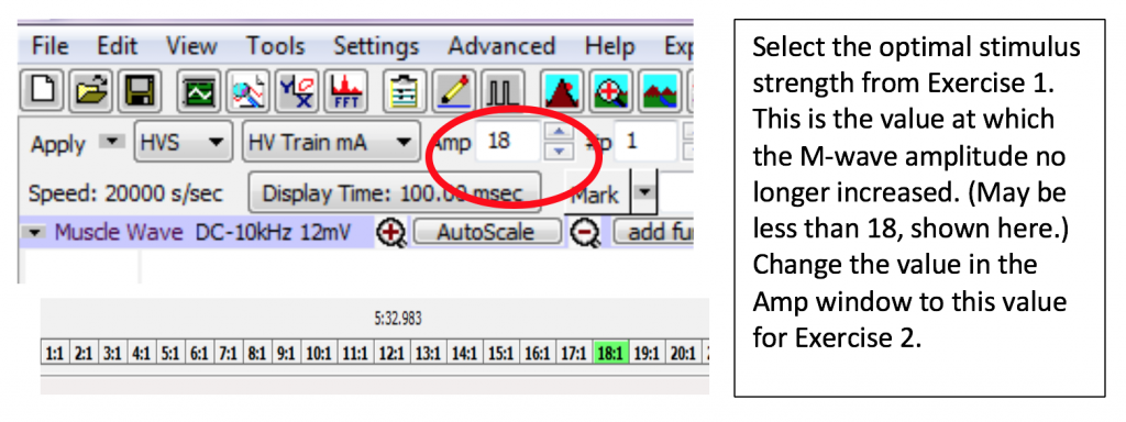
Exercise 1: Stimulus Strength and Muscle Response
Objective: To determine the effect of stimulus strength on the response of the innervated abductor digiti minimi muscle.
Overview: You will stimulate the abductor digiti minimi motor neuron with increasing amounts of current (measured in milliAmps, read as AMP on LabScribe). You will measure the EMG muscle response each time (in mV) and record the value in your lab report. You will continue until you get three readings in a row with the same value (+/- 0.2 mV). Of those three readings, put a mark next to the lowest current (Amplitude) value on your lab report; you will be using this value for exercise 2.
Checking electrode placement and preparing to record data
- Ask the subject to place his or her right hand on the bench with the palm down or let hang relaxed at their side. Tell the subject to relax. Note: The subject should make sure to relax his/her forearm and hand completely. At the beginning, you will need to continue to increase the pulse amplitude until a response is generated. Stimulus that does not create a muscle contraction is subthreshold.
- When starting this experiment, check to make sure 0 is the number in the AMP Window. If it is not, please change the value to zero. Click Record button on the LabScribe Main window. LabScribe will record a single sweep with a display time of 50 milliseconds. Since the output amplitude is set to zero, there should be no response from the abductor digiti muscle (no muscle twitch in the pinky finger).
- Increase the output amplitude to 1 milliAmp on the Tool Bar by using the up/down arrows or placing 1 in the box by highlighting and changing the number to 1 (AMP). Click “APPLY”. Click the Record button again and record another sweep. Click the AutoScale button for the Muscle channel to improve the display of the muscle’s response (Methods Figure 1).
Continue to increase the output amplitude by an increment of 1 mAMP (1 “AMP” on the LabScribe stimulator button) until you get a muscle twitch and EMG M-wave for the subject. Click apply.
Remember, after each increase in amplitude, you must click “APPLY” before doing another recording!
-
- 1 AMP – APPLY – Record
- 2 AMP – APPLY – Record
- 3 AMP – APPLY – Record
- 4 AMP – APPLY – Record…etc.
- If you get no Action Potential Wave on the EMG screen by 10 AMP, reposition the electrode pads starting with D.
- Keep the snaps in line and move D & E slightly to one side of the previous position.
- Ask your TA for help.
Start data collection for Experiment 1
- Now that we know the electrode placement is optimal, open a new data file. EACH PARTICIPANT should have their own data file for this lab.
- Go back to AMP 1 to start collecting data.
- After recording each “sweep” (each time you click RECORD), immediately perform the data analysis on the Main Window (see below). Do not record all sweeps and go back to do analysis, as it may make longer.
- Continue to increase the output amplitude by 1 AMP always clicking “APPLY” and then recording the response until the muscle impulse reaches a maximum (the amplitude of the M Wave peaks from your analysis no longer increases with additional applied stimulus): once you get three readings in a row with the same value (+/- 0.2 mV), note the lowest of the three AMP values. You will be using this value for exercise 2. A maximum of 19 is possible; do not go past 19 AMP.
- When you are done, be sure to select Save As in the File menu and name the file. Choose a destination on the computer in which to save the file (e.g. your folder). Click the Save button to save the file (as an *.iwxdata file).
Exercise 1 Data Analysis
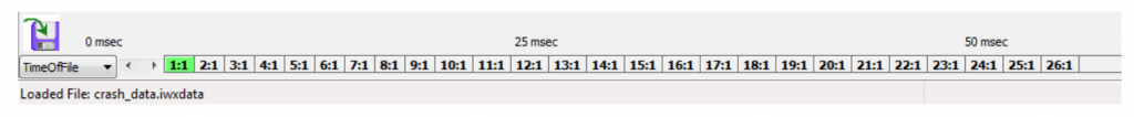
Different sweeps may be selected any time by clicking on the Sweeps list on the bottom of the Main Screen (1:1, 2:1, etc.). If analyzing data on the Main Screen while recording, the sweep you need to analyze is already selected. The Sweeps task bar is shown below.
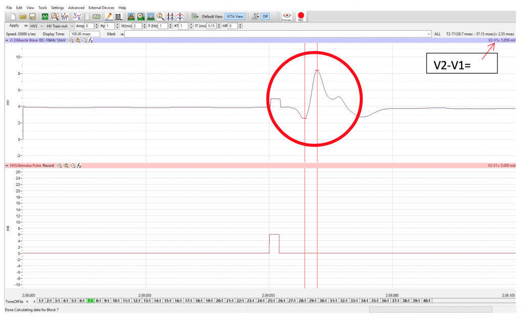
- Record V2-V1, the M-Wave amplitude
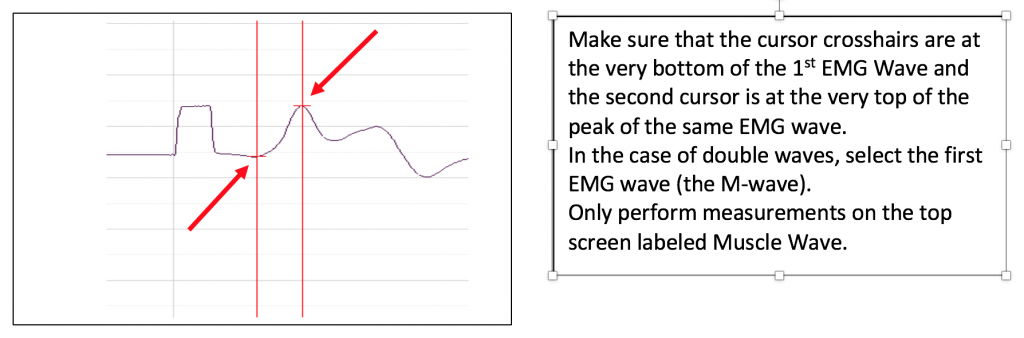
- To find the amplitude: Click and Drag one cursor to the base of the EMG wave and the second cursor to the top peak EMG wave. In the case of multiple waves select the first EMG wave (not the stimulus artifact), the M-wave is shown in the picture, below. The value V2-V1 found in the table at the top right of the Main window is the amplitude of the muscle response. Record the amplitude of each response (in mV) with its corresponding applied stimulus strength (in mA) in the table in your lab report. Measure all visible EMG Waves (action potentials). If there is no EMG M-Wave record “Subthreshold” on your lab report.
Exercise 2: Ulnar Nerve Conduction Velocity
Objective: To measure the conduction velocity (transmission speed) of the ulnar nerve.
Overview
You will use the AMP value which excited the maximal response in experiment 1 and stimulate the same abductor digiti minimi motor neuron further up the arm. You will then use that previous experiment and the one you will conduct here to compare the time between innervation and the elicitation of the response for two points on the nerve. You will measure the distance between the stimulation electrodes and calculate the transmission speed in m/s.
Procedure
- Ask the subject to place his or her right hand on the bench with the palm down. Tell the subject to relax.
- Move the red (+) stimulating lead from Electrode E to Electrode G, and the black (-) stimulating lead from Electrode D to Electrode F. Video available on the P-Drive.
Test the placement by setting the Amplitude to the number that produced the optimal Action Potential previously. Click Apply and Click Record. If you get an Action Potential on the EMG screen proceed to Step 1 below.
If you do not get an Action Potential, reposition F and G electrode pads and test again. Ask your TA for help. Reposition the stimulator electrodes until you get an Action Potential then proceed to step 1 below.
- Set the Amplitude on the Labscribe toolbar to the first AMP value that delivered a maximal muscle response in Exercise 1. Click Apply.
- Click the Record button on the LabScribe Main window to record a single sweep at this stimulus strength.
- Select Save in the File menu.
- Use a tape measure and measure the actual distance, in millimeters, between the placement of the black (-) stimulating electrodes (Electrodes D and F) in exercises 1 and 2: Measure from the center of the snap on D to the center of the black stimulator on F, in a straight line.
Exercise 2 Data Analysis
- Click on Double Cursors.
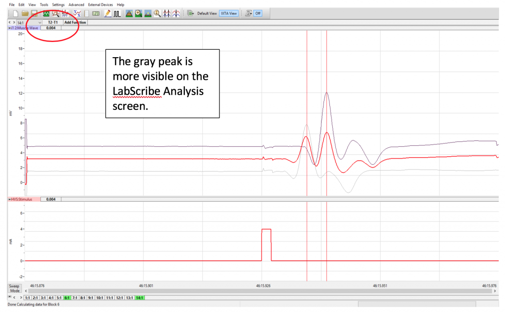
- Click the Analysis icon in the LabScribe toolbar to view the recorded sweeps. From the Sweeps list, select the sweep that had delivered the maximal muscle response in Exercise 1, along with the sweep from Exercise 2. This will superimpose the sweeps on each other (see Methods Fig. 6, below). The Red line is the algebraic sum of both, ignore that line.
- Now measure peak to peak by placing one cursor on the M-wave peak of the gray line and the other cursor on the M-wave peak of the black line. If the cursors do not move and stay where you want them Click the Double Cursor again.
- If T2-T1 are not on the Tool Bar, select add function on the Tool Bar, then General on the drop-down menu and then select T2-T1.
- The value for T2-T1 displayed in the Tool Bar on the Analysis window is the difference in response time between the two positions of the negative stimulating electrode (e.g. it takes longer to elicit the M-wave the further the stimulating electrodes are from the muscle being measured). Note that the time on the Analysis Tool Bar is in seconds and you need to convert it to milliseconds. (example, 0.004sec = 4ms)
- Calculate the conduction velocity (in m/sec) by dividing the distance (in mm) between the two positions of the negative stimulating electrode by the time (T2-T1) between the peaks of the muscle responses from those two positions.
- For example:225 mm between positions of (-) electrode / 4 ms = 56.25mm/ms = 56.25m/sReport the velocity and show all your calculations on your lab report.
Please cite:
Haen Whitmer, K.M. (2021). A Mixed Course-Based Research Approach to Human Physiology. Ames, IA: Iowa State University Digital Press. https://iastate.pressbooks.pub/curehumanphysiology/
