
3 CIRCUIT TOPOLOGY AND LAWS
3.1 Simple Series Circuits
On this page, we’ll outline the three principles you should understand regarding series circuits:
Current: The amount of current is the same through any component in a series circuit.
Resistance: The total resistance of any series circuit is equal to the sum of the individual resistances.
Voltage: The supply voltage in a series circuit is equal to the sum of the individual voltage drops.
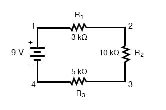
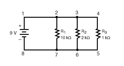
Let’s take a look at some examples of series circuits that demonstrate these principles. We’ll start with a series circuit consisting of three resistors and a single battery:
The first principle to understand about series circuits is as follows:
The amount of current in a series circuit is the same through any component in the circuit.
Total Series Current
[latex]\tag{3.1} I_{Total} = I_1 = I_2 = ...=I_n[/latex]
This is because there is only one path for current flow in a series circuit. Because electric charge flows through conductors like marbles in a tube, the rate of flow (marble speed) at any point in the circuit (tube) at any specific point in time must be equal.
3.2 Using Ohm’s Law in Series Circuits
From the way that the 9 volt battery is arranged, we can tell that the current in this circuit will flow in a clockwise direction, from point 1 to 2 to 3 to 4 and back to 1. However, we have one source of voltage and three resistances. How do we use Ohm’s Law here?
An important caveat to Ohm’s Law is that all quantities (voltage, current, resistance, and power) must relate to each other in terms of the same two points in a circuit. We can see this concept in action in the single resistor circuit example below.
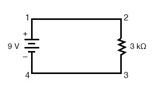
Using Ohm’s Law in a Simple, Single Resistor Circuit
With a single-battery, single-resistor circuit, we could easily calculate any quantity because they all applied to the same two points in the circuit:
[latex]I\:=\frac{E}{R}[/latex]
[latex]I\:=\frac{9V}{3k\Omega}[/latex]
[latex]\pmb{I = 3 mA}[/latex]
Since points 1 and 2 are connected together with the wire of negligible resistance, as are points 3 and 4, we can say that point 1 is electrically common to point 2, and that point 3 is electrically common to point 4. Since we know we have 9-volt of electromotive force between points 1 and 4 (directly across the battery), and since point 2 is common to point 1 and point 3 common to point 4, we must also have 9-volt between points 2 and 3 (directly across the resistor).
Therefore, we can apply Ohm’s Law (I= E/R) to the current through the resistor, because we know the voltage (E) across the resistor and the resistance (R) of that resistor. All terms (E, I, R) apply to the same two points in the circuit, to that same resistor, so we can use the Ohm’s Law formula with no reservation.
Using Ohm’s Law in Circuits with Multiple Resistors
In circuits containing more than one resistor, we must be careful in how we apply Ohm’s Law. In the three-resistor example circuit below, we know that we have 9 volts between points 1 and 4, which is the amount of electromotive force driving the current through the series combination of R1, R2, and R3 . However, we cannot take the value of 9-volt and divide it by 3k, 10k or 5k Ω to try to find a current value, because we don’t know how much voltage is across any one of those resistors, individually.
The figure of 9 volts is a total quantity for the whole circuit, whereas the figures of 3k, 10k, and 5k Ω are individual quantities for individual resistors. If we were to plug a figure for total voltage into an Ohm’s Law equation with a figure for individual resistance, the result would not relate accurately to any quantity in the real circuit.
For R1, Ohm’s Law will relate the amount of voltage across R1 with the current through R1, given R1‘s resistance, 3kΩ:
But, since we don’t know the voltage across R1 (only the total voltage supplied by the battery across the three-resistor series combination) and we don’t know the current through R1, we can’t do any calculations with either formula. The same goes for R2 and R3: we can apply the Ohm’s Law equations if and only if all terms are representative of their respective quantities between the same two points in the circuit.
So what can we do? We know the voltage of the source (9 volts) applied across the series combination of R1, R2, and R3, and we know the resistance of each resistor, but since those quantities aren’t in the same context, we can’t use Ohm’s Law to determine the circuit current. If only we knew what the total resistance was for the circuit: then we could calculate the total current with our figure for total voltage (I=E/R).
Combining Multiple Resistors into an Equivalent Total Resistor
This brings us to the second principle of series circuits:
The total resistance of any series circuit is equal to the sum of the individual resistances.
This should make intuitive sense: the more resistors in series that the current must flow through, the more difficult it will be for the current to flow.
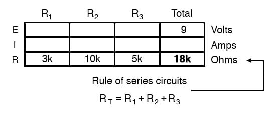
In the example problem, we had a 3 kΩ, 10 kΩ, and 5 kΩ resistors in series, giving us a total resistance of 18 kΩ:

[latex]R_{total} = R_1 + R_2 + R_3[/latex]
[latex]R_{total} = 3\text{ k}\Omega + 10\text{ k}\Omega + 5 \text{ k}\Omega[/latex]
[latex]\pmb{R_{total} = 18\text{ k}\Omega}[/latex]
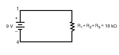
In essence, we’ve calculated the equivalent resistance of R1, R2, and R3 combined. Knowing this, we could redraw the circuit with a single equivalent resistor representing the series combination of R1, R2, and R3:
Calculating Circuit Current Using Ohm’s Law
Now we have all the necessary information to calculate circuit current because we have the voltage between points 1 and 4 (9 volts) and the resistance between points 1 and 4 (18 kΩ):
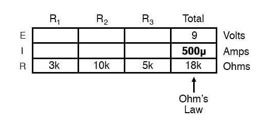
[latex]I_{total}\:=\frac{E_{total}}{R_{total}}[/latex]
[latex]\:=\frac{9V}{18k\Omega}[/latex]
[latex]\pmb{I_{total}= 500µA}[/latex]
Calculating Component Voltages Using Ohm’s Law
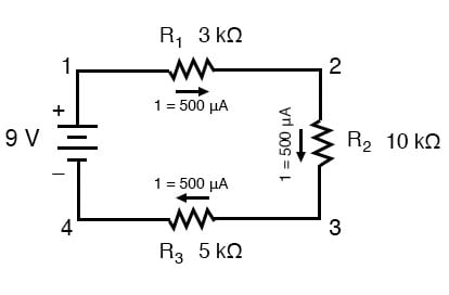
Knowing that current is equal through all components of a series circuit (and we just determined the current through the battery), we can go back to our original circuit schematic and note the current through each component:
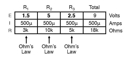
Now that we know the amount of current through each resistor, we can use Ohm’s Law to determine the voltage drop across each one (applying Ohm’s Law in its proper context):
[latex]E_{R1} = I_{R1}{R_1}[/latex]
[latex]= (500µA){(3kΩ)}[/latex]
[latex]\pmb{E_{R1}=1.5V}[/latex]
[latex]E_{R2} = I_{R2}{R_2}[/latex]
[latex]= (500µA){(10kΩ)}[/latex]
[latex]\pmb{E_{R2}=5V}[/latex]
[latex]E_{R3} = I_{R3}{R_3}[/latex]
[latex]= (500µA){(5kΩ)}[/latex]
[latex]\pmb{E_{R3}=2.5V}[/latex]
Notice the voltage drops across each resistor, and how the sum of the voltage drops (1.5 + 5 + 2.5) is equal to the battery (supply) voltage: 9 volts.
This is the third principle of series circuits:
The supply voltage in a series circuit is equal to the sum of the individual voltage drops.
Total Series Voltage
[latex]E_{total} = E_1 + E_2 +... E_n \tag{3.3}[/latex]
Analyzing Simple Series Circuits with the “Table Method” and Ohm’s Law
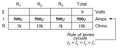
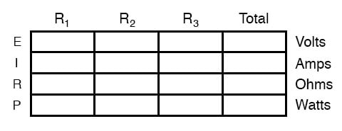
However, the method we just used to analyze this simple series circuit can be streamlined for better understanding. By using a table to list all voltages, currents, and resistance in the circuit, it becomes very easy to see which of those quantities can be properly related in any Ohm’s Law equation:
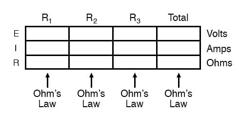
The rule with such a table is to apply Ohm’s Law only to the values within each vertical column. For instance, ER1 only with IR1 and R1; ER2 only with IR2 and R2; etc. You begin your analysis by filling in those elements of the table that are given to you from the beginning:
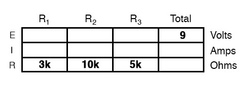
As you can see from the arrangement of the data, we can’t apply the 9 volts of ET (total voltage) to any of the resistances (R1, R2, or R3) in any Ohm’s Law formula because they’re in different columns. The 9 volts of battery voltage is not applied directly across R1, R2, or R3. However, we can use our “rules” of series circuits to fill in blank spots on a horizontal row. In this case, we can use the series rule of resistances to determine a total resistance from the sum of individual resistances:
Now, with a value for total resistance inserted into the rightmost (“Total”) column, we can apply Ohm’s Law of I=E/R to total voltage and total resistance to arrive at a total current of 500 µA:
Then, knowing that the current is shared equally by all components of a series circuit (another “rule” of series circuits), we can fill in the currents for each resistor from the current figure just calculated:
Finally, we can use Ohm’s Law to determine the voltage drop across each resistor, one column at a time:
In summary, a series circuit is defined as having only one path through which current can flow. From this definition, three rules of series circuits follow: all components share the same current; resistances add to equal a larger, total resistance; and voltage drops add to equal a larger, total voltage. All of these rules find root in the definition of a series circuit. If you understand that definition fully, then the rules are nothing more than footnotes to the definition.
- Components in a series circuit share the same current:
[latex]I_{Total} = I_1 = I_2 = I_3= ... =I_n[/latex]
- The total resistance in a series circuit is equal to the sum of the individual resistances:
[latex]R_{Total} = R_1 + R_2 + ...+ R_n[/latex]
- Total voltage in a series circuit is equal to the sum of the individual voltage drops:
[latex]E_{Total} = E_1 + E_2 +... +E_n[/latex]
3.3 Simple Parallel Circuits
In this section, we’ll outline the three principles you should understand regarding parallel circuits:
Voltage: Voltage is equal across all components in a parallel circuit.
Current: The total circuit current is equal to the sum of the individual branch currents.
Resistance: Individual resistances diminish to equal a smaller total resistance rather than add to make the total.
Let’s take a look at some examples of parallel circuits that demonstrate these principles.
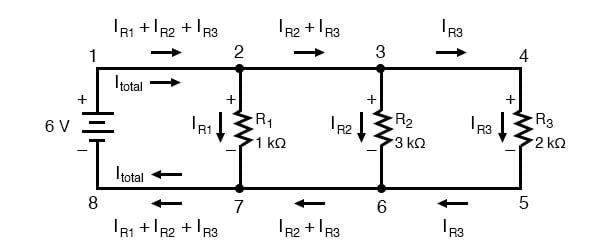
We’ll start with a parallel circuit consisting of three resistors and a single battery:
Voltage in Parallel Circuits
The first principle to understand about parallel circuits is that the voltage is equal across all components in the circuit. This is because there are only two sets of electrically common points in a parallel circuit, and the voltage measured between sets of common points must always be the same at any given time.
Therefore, in the above circuit, the voltage across R1 is equal to the voltage across R2 which is equal to the voltage across R3 which is equal to the voltage across the battery.
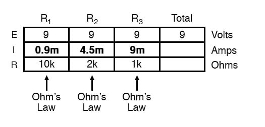
This equality of voltages can be represented in another table for our starting values:
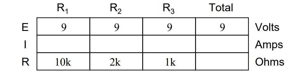
Ohm’s Law Applications for Simple Parallel Circuits
Just as in the case of series circuits, the same caveat for Ohm’s Law applies: values for voltage, current, and resistance must be in the same context in order for the calculations to work correctly.
However, in the above example circuit, we can immediately apply Ohm’s Law to each resistor to find its current because we know the voltage across each resistor (9 volts) and the resistance of each resistor:
[latex]I_{R1}\:=\frac{E_{R1}}{R_1}[/latex]
[latex]\:=\frac{(9V)}{(10kΩ)}[/latex]
[latex]\pmb{I_{R1}\:=0.9mA}[/latex]
[latex]I_{R2}\:=\frac{E_{R2}}{R_2}[/latex]
[latex]\:=\frac{(9V)}{(2kΩ)}[/latex]
[latex]\pmb{I_{R2}\:=4.5mA}[/latex]
[latex]I_{R3}\:=\frac{E_{R3}}{R_3}[/latex]
[latex]\:=\frac{(9V)}{(1kΩ)}[/latex]
[latex]\pmb{I_{R3}=9mA}[/latex]
At this point, we still don’t know what the total current or total resistance for this parallel circuit is, so we can’t apply Ohm’s Law to the rightmost (“Total”) column. However, if we think carefully about what is happening, it should become apparent that the total current must equal the sum of all individual resistor (“branch”) currents:
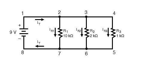
As the total current exits the positive (+) battery terminal at point 1 and travels through the circuit, some of the flow splits off at point 2 to go through R1, some more splits off at point 3 to go through R2, and the remainder goes through R3. Like a river branching into several smaller streams, the combined flow rates of all streams must equal the flow rate of the whole river.
The same thing is encountered where the currents through R1, R2, and R3 join to flow back to the negative terminal of the battery (-) toward point 8: the flow of current from point 7 to point 8 must equal the sum of the (branch) currents through R1, R2, and R3.
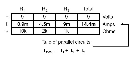
This is the second principle of parallel circuits: the total circuit current is equal to the sum of the individual branch currents.
Using this principle, we can fill in the IT spot on our table with the sum of IR1, IR2, and IR3:
How to Calculate Total Resistance in Parallel Circuits
Finally, applying Ohm’s Law to the rightmost (“Total”) column, we can calculate the total circuit resistance:
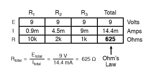
The Equation for Resistance in Parallel Circuits
Please note something very important here. The total circuit resistance is only 625 Ω: less than any one of the individual resistors. In the series circuit, where the total resistance was the sum of the individual resistances, the total was bound to be greater than anyone of the resistors individually.
Here in the parallel circuit, however, the opposite is true: we say that the individual resistances diminish rather than add to make the total.
This principle completes our triad of “rules” for parallel circuits, just as series circuits were found to have three rules for voltage, current, and resistance.
Mathematically, the relationship between total resistance and individual resistances in a parallel circuit looks like this:
The Equation for Resistance in Parallel Circuits
[latex]R_{total}=\frac{1}{\frac{1}{R_1}+\frac{1}{R_2}+...+\frac{1}{R_n}}\tag{3.5}[/latex]
Three Rules of Parallel Circuits
In summary, a parallel circuit is defined as one where all components are connected between the same set of electrically common points. Another way of saying this is that all components are connected across each other’s terminals.
From this definition, three rules of parallel circuits follow:
All components share the same voltage.
Resistances diminish to equal a smaller, total resistance.
Branch currents add to equal a larger, total current.
Just as in the case of series circuits, all of these rules find root in the definition of a parallel circuit. If you understand that definition fully, then the rules are nothing more than footnotes to the definition.
- Components in a parallel circuit share the same voltage:
[latex]E_{Total} = E_1 = E_2= ...=E_n[/latex]
- Total resistance in a parallel circuit is less than any of the individual resistances:
[latex]R_{Total}=\frac{1}{\frac{1}{R_1}+\frac{1}{R_2}+...+\frac{1}{R_n}}[/latex]
- Total current in a parallel circuit is equal to the sum of the individual branch currents:
[latex]I_{Total} = I_1 +I_2+ ...+I_n[/latex]
3.4 Power Calculations
When calculating the power dissipation of resistive components, use any one of the three power equations to derive the answer from values of voltage, current, and/or resistance pertaining to each component:
Power Equation
[latex]P = {IE}[/latex]
[latex]P=\frac{E^2}{R}[/latex]
[latex]P = {I^2R}[/latex]
This is easily managed by adding another row to our familiar table of voltages, currents, and resistances:
Power for any particular table column can be found by the appropriate Ohm’s Law equation (appropriate based on what figures are present for E, I, and R in that column).
An interesting rule for total power versus individual power is that it is additive for any configuration of the circuit: series, parallel, series/parallel, or otherwise. Power is a measure of the rate of work, and since power dissipated must equal the total power applied by the source(s) (as per the Law of Conservation of Energy in physics), circuit configuration has no effect on the mathematics.
- Power is additive in any configuration of resistive circuit:
[latex]P_{Total} = P_1 +P_2+ ...+P_n[/latex]
3.5 Correct use of Ohm’s Law
Reminders When Using Ohm’s Law
One of the most common mistakes made by beginning electronics students in their application of Ohm’s Laws is mixing the contexts of voltage, current, and resistance. In other words, a student might mistakenly use a value for I (current) through one resistor and the value for E (voltage) across a set of interconnected resistors, thinking that they’ll arrive at the resistance of that one resistor.
Not so! Remember this important rule: The variables used in Ohm’s Law equations must be common to the same two points in the circuit under consideration. I cannot overemphasize this rule. This is especially important in series-parallel combination circuits where nearby components may have different values for both voltage drop and current.
When using Ohm’s Law to calculate a variable pertaining to a single component, be sure the voltage you’re referencing is sole across that single component and the current you’re referencing is solely through that single component and the resistance you’re referencing is solely for that single component. Likewise, when calculating a variable pertaining to a set of components in a circuit, be sure that the voltage, current, and resistance values are specific to that complete set of components only!
A good way to remember this is to pay close attention to the two points terminating the component or set of components being analyzed, making sure that the voltage in question is across those two points, that the current in question is the flow of electric charge from one of those points all the way to the other point, that the resistance in question is the equivalent of a single resistor between those two points, and that the power in question is the total power dissipated by all components between those two points.
Notes on the “Table” Method of Analyzing Circuits
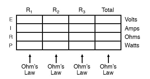
The “table” method presented for both series and parallel circuits in this chapter is a good way to keep the context of Ohm’s Law correct for any kind of circuit configuration. In a table like the one shown below, you are only allowed to apply an Ohm’s Law equation for the values of a single vertical column at a time:
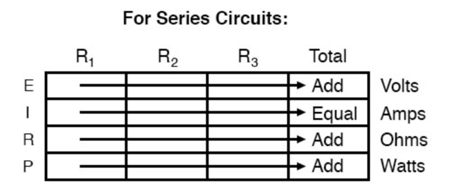
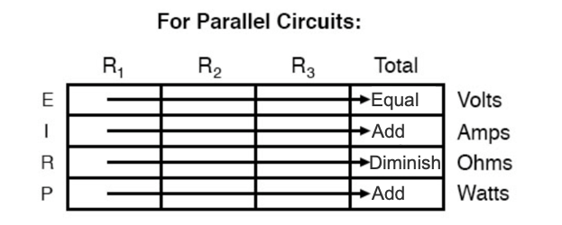
Deriving values horizontally across columns is allowable as per the principles of series and parallel circuits:
Not only does the “table” method simplifies the management of all relevant quantities, but it also facilitates cross-checking of answers by making it easy to solve for the original unknown variables through other methods, or by working backward to solve for the initially given values from your solutions. For example, if you have just solved for all unknown voltages, currents, and resistance in a circuit, you can check your work by adding a row at the bottom for power calculations on each resistor, seeing whether or not all the individual power values add up to the total power. If not, then you must have made a mistake somewhere! While this technique of “cross-checking” your work is nothing new, using the table to arrange all the data for the cross-check(s) results in a minimum of confusion.
- Apply Ohm’s Law to vertical columns in the table.
- Apply rules of series/parallel to horizontal rows in the table.
- Check your calculations by working “backward” to try to arrive at originally given values (from your first calculated answers), or by solving for a quantity using more than one method (from different given values).
3.6 Kirchhoff’s Voltage Law (KVL)
What is Kirchhoff’s Voltage Law (KVL)?
The principle known as Kirchhoff’s Voltage Law (discovered in 1847 by Gustav R. Kirchhoff, a German physicist) can be stated as such:
“The algebraic sum of all voltages in a loop must equal zero”
[latex]E_{T} = E_1 + E_2 +... +E_n= 0[/latex]
By algebraic, I mean accounting for signs (polarities) as well as magnitudes. By loop, I mean any path traced from one point in a circuit around to other points in that circuit, and finally back to the initial point.
Demonstrating Kirchhoff’s Voltage Law in a Series Circuit
Let’s take another look at our example series circuit, this time numbering the points in the circuit for voltage reference:
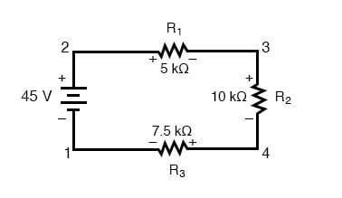
If we were to connect a voltmeter between points 2 and 1, the red test leads to point 2 and the black test lead to point 1, the meter would register +45 volts. Typically, the “+” sign is not shown but rather implied, for positive readings in digital meter displays. However, for this lesson, the polarity of the voltage reading is very important and so I will show positive numbers explicitly: E2-1 = +45V
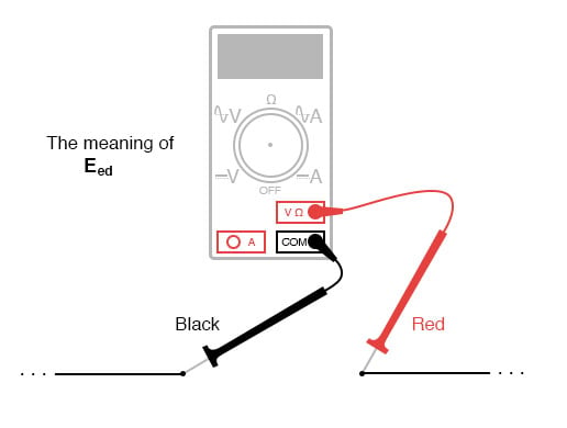
When a voltage is specified with a double subscript (the characters “2-1” in the notation “E2-1”), it means the voltage at the first point (2) as measured in reference to the second point (1). A voltage specified as “Ecd” would mean the voltage as indicated by a digital meter with the red test lead on point “c” and the black test lead on point “d”: the voltage at “c” in reference to “d”.
If we were to take that same voltmeter and measure the voltage drop across each resistor, stepping around the circuit in a clockwise direction with the red test lead of our meter on the point ahead and the black test lead on the point behind, we would obtain the following readings:
[latex]E_{3-2} = -10V[/latex]
[latex]E_{4-3} = -20V[/latex]
[latex]E_{1-4} = -15V[/latex]
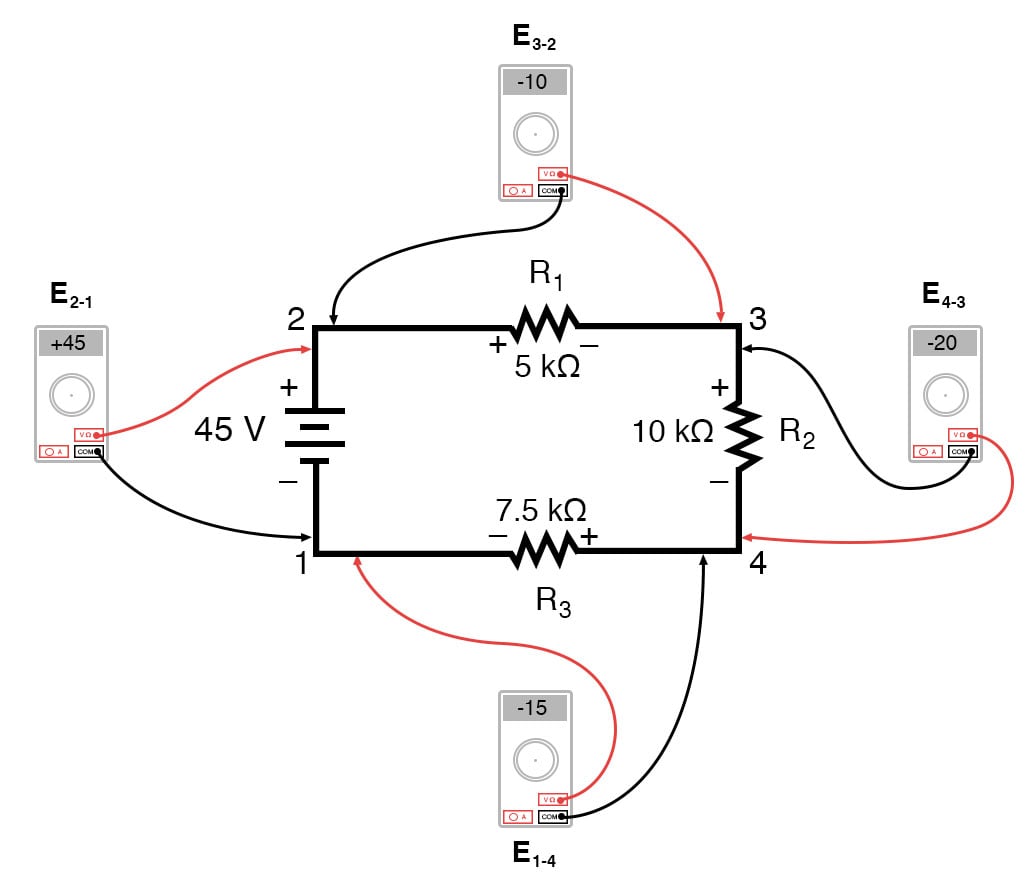
We should already be familiar with the general principle for series circuits stating that individual voltage drops add up to the total applied voltage, but measuring voltage drops in this manner and paying attention to the polarity (mathematical sign) of the readings reveals another facet of this principle: that the voltages measured as such all add up to zero:
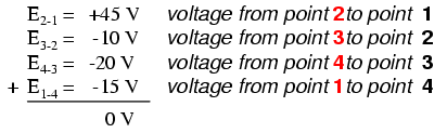
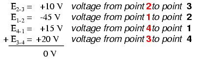
In the above example, the loop was formed by the following points in this order: 1-2-3-4-1. It doesn’t matter which point we start at or which direction we proceed in tracing the loop; the voltage sum will still equal zero. To demonstrate, we can tally up the voltages in loop 3-2-1-4-3 of the same circuit:
This may make more sense if we re-draw our example series circuit so that all components are represented in a straight line:

It’s still the same series circuit, just with the components arranged in a different form. Notice the polarities of the resistor voltage drops with respect to the battery: the battery’s voltage is negative on the left and positive on the right, whereas all the resistor voltage drops are oriented the other way: positive on the left and negative on the right. This is because the resistors are resisting the flow of electric charge being pushed by the battery. In other words, the “push” exerted by the resistors against the flow of electric charge must be in a direction opposite the source of electromotive force.
Here we see what a digital voltmeter would indicate across each component in this circuit, black lead on the left and red lead on the right, as laid out in horizontal fashion:

If we were to take that same voltmeter and read voltage across combinations of components, starting with the only R1 on the left and progressing across the whole string of components, we will see how the voltages add algebraically (to zero):
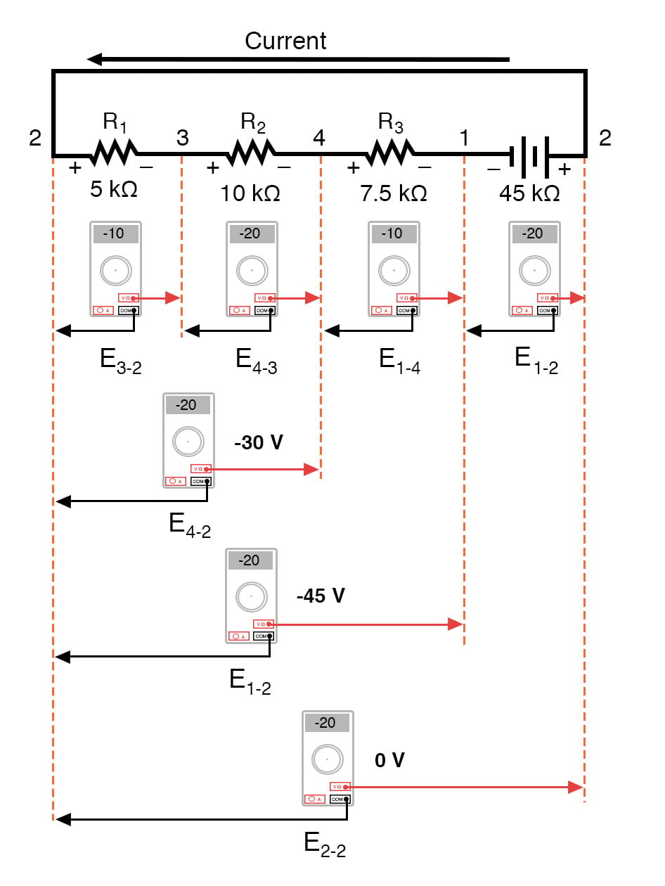
The fact that series voltages add up should be no mystery, but we notice that the polarity of these voltages makes a lot of difference in how the figures add. While reading voltage across R1—R2, and R1—R2—R3(I’m using a “double-dash” symbol “—” to represent the series connection between resistors R1, R2, and R3), we see how the voltages measure successively larger (albeit negative) magnitudes, because the polarities of the individual voltage drops are in the same orientation (positive left, negative right). The sum of the voltage drops across R1, R2, and R3 equals 45 volts, which is the same as the battery’s output, except that the battery’s polarity is opposite that of the resistor voltage drops (negative left, positive right), so we end up with 0 volts measured across the whole string of components.
That we should end up with exactly 0 volts across the whole string should be no mystery, either. Looking at the circuit, we can see that the far left of the string (left side of R1: point number 2) is directly connected to the far right of the string (right side of battery: point number 2), as necessary to complete the circuit. Since these two points are directly connected, they are electrically common to each other. And, as such, the voltage between those two electrically common points must be zero.
Demonstrating Kirchhoff’s Voltage Law in a Parallel Circuit
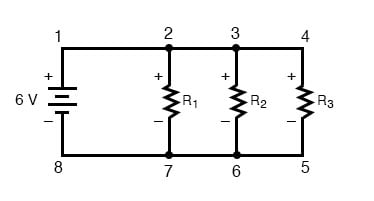
Kirchhoff’s Voltage Law (sometimes denoted as KVL for short) will work for any circuit configuration at all, not just a simple series. Note how it works for this parallel circuit:
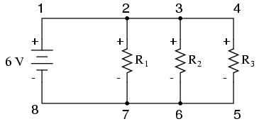
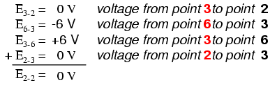
Being a parallel circuit, the voltage across every resistor is the same as the supply voltage: 6 volts. Tallying up voltages around loop 2-3-4-5-6-7-2, we get:
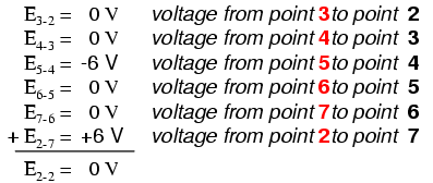
Note how I label the final (sum) voltage as E2-2. Since we began our loop-stepping sequence at point 2 and ended at point 2, the algebraic sum of those voltages will be the same as the voltage measured between the same point (E2-2), which of course must be zero.
The Validity of Kirchhoff’s Voltage Law, Regardless of Circuit Topology
The fact that this circuit is parallel instead of series has nothing to do with the validity of Kirchhoff’s Voltage Law. For that matter, the circuit could be a “black box”—its component configuration completely hidden from our view, with only a set of exposed terminals for us to measure the voltage between—and KVL would still hold true:
Try any order of steps from any terminal in the above diagram, stepping around back to the original terminal, and you’ll find that the algebraic sum of the voltages always equals zero.
Furthermore, the “loop” we trace for KVL doesn’t even have to be a real current path in the closed-circuit sense of the word. All we have to do to comply with KVL is to begin and end at the same point in the circuit, tallying voltage drops and polarities as we go between the next and the last point. Consider this absurd example, tracing “loop” 2-3-6-3-2 in the same parallel resistor circuit:
Using Kirchhoff’s Voltage Law in a Complex Circuit
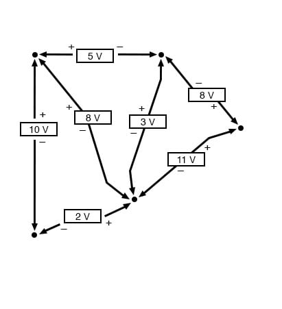
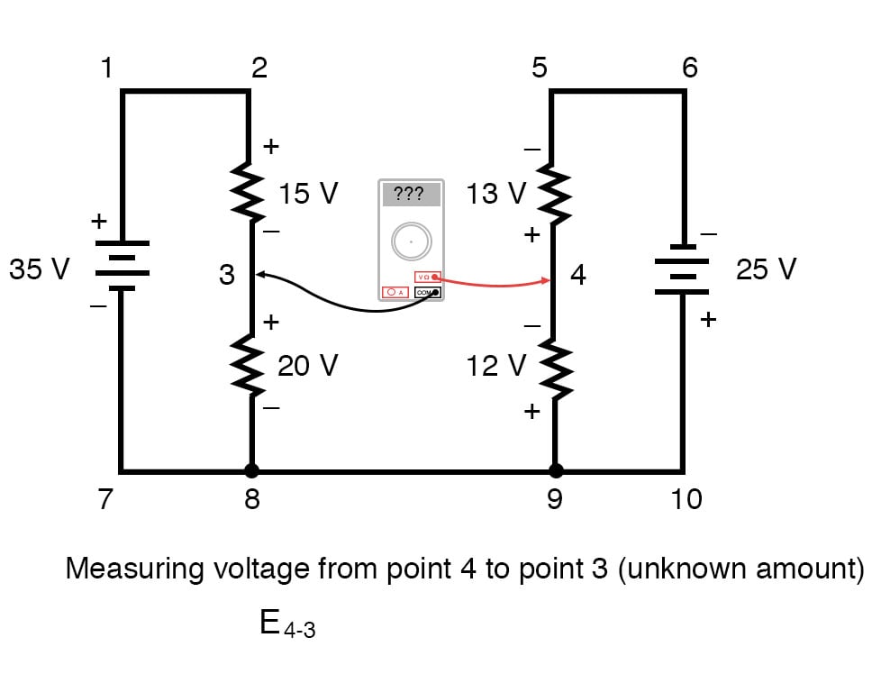
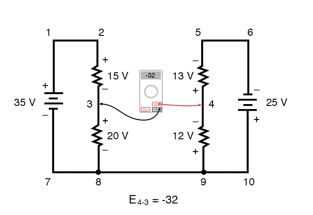
KVL can be used to determine an unknown voltage in a complex circuit, where all other voltages around a particular “loop” are known. Take the following complex circuit (actually two series circuits joined by a single wire at the bottom) as an example:
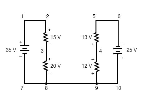
To make the problem simpler, I’ve omitted resistance values and simply given voltage drops across each resistor. The two series circuits share a common wire between them (wire 7-8-9-10), making voltage measurements between the two circuits possible.
If we wanted to determine the voltage between points 4 and 3, we could set up a KVL equation with the voltage between those points as the unknown:
[latex]E_{4-3} +E_{9-4} +E_{8-9} +E_{3-8}= 0[/latex]
[latex]E_{4-3} +12V+0V +20V= 0V[/latex]
[latex]E_{4-3} +32V = 0[/latex]
[latex]\pmb{E_{4-3} = -32V}[/latex]
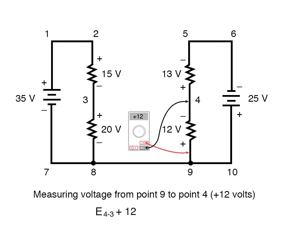
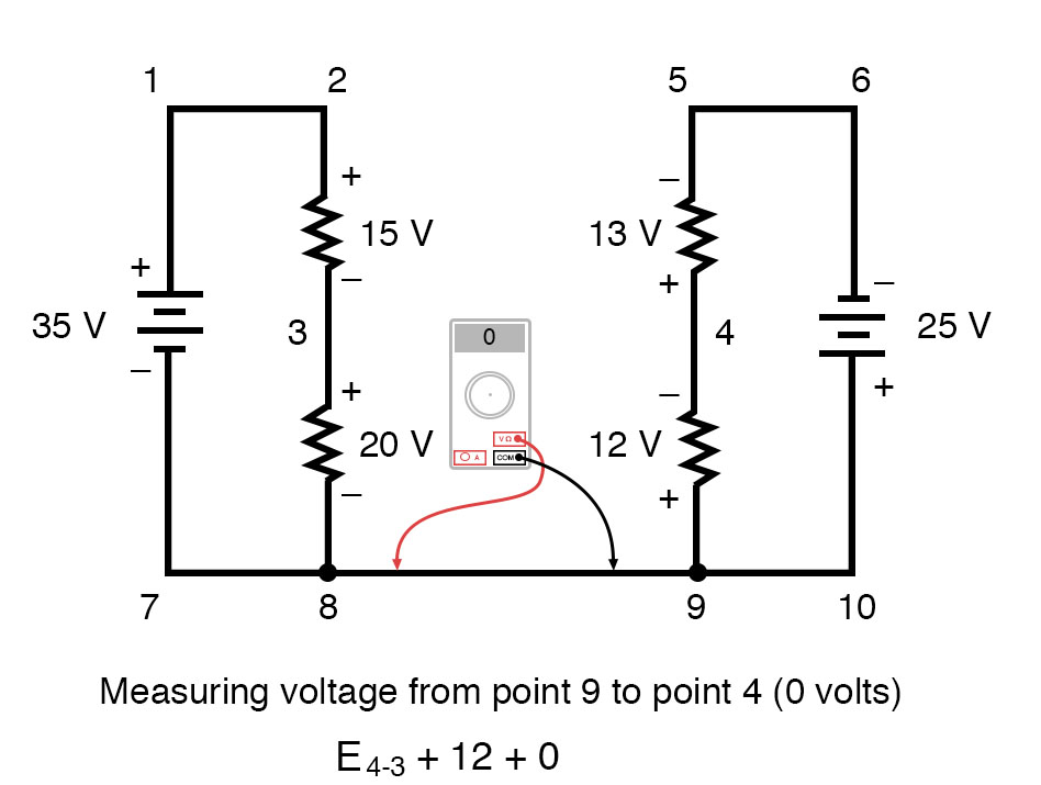
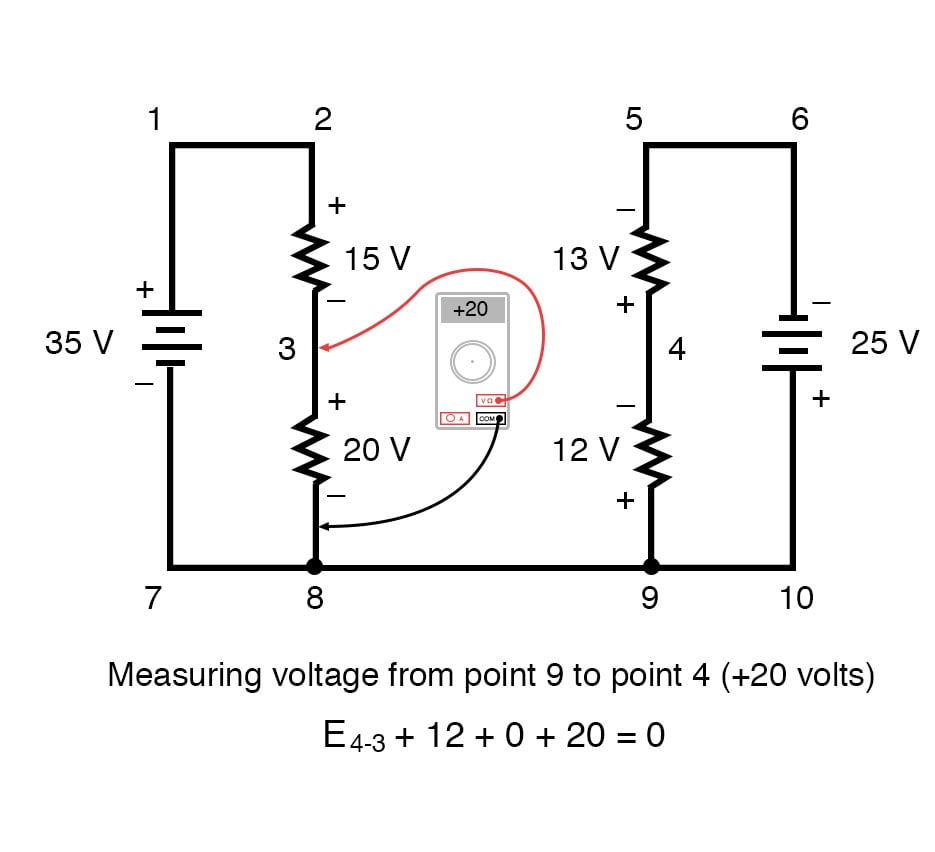
Stepping around the loop 3-4-9-8-3, we write the voltage drop figures as a digital voltmeter would register them, measuring with the red test lead on the point ahead and black test lead on the point behind as we progress around the loop. Therefore, the voltage from point 9 to point 4 is a positive (+) 12 volts because the “red lead” is on point 9 and the “black lead” is on point 4. The voltage from point 3 to point 8 is a positive (+) 20 volts because the “red lead” is on point 3 and the “black lead” is on point 8. The voltage from point 8 to point 9 is zero, of course, because those two points are electrically common.
Our final answer for the voltage from point 4 to point 3 is a negative (-) 32 volts, telling us that point 3 is actually positive with respect to point 4, precisely what a digital voltmeter would indicate with the red lead on point 4 and the black lead on point 3:
In other words, the initial placement of our “meter leads” in this KVL problem was “backward.” Had we generated our KVL equation starting with E3-4 instead of E4-3, stepping around the same loop with the opposite meter lead orientation, the final answer would have been E3-4 = +32 volts:
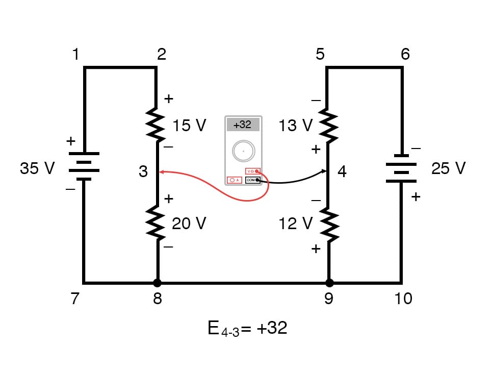
It is important to realize that neither approach is “wrong.” In both cases, we arrive at the correct assessment of voltage between the two points, 3 and 4: point 3 is positive with respect to point 4, and the voltage between them is 32 volts.
- Kirchhoff’s Voltage Law (KVL): “The algebraic sum of all voltages in a loop must equal zero”
3.7 Kirchhoff’s Current Law (KCL)
What is Kirchhoff’s Current Law?
Kirchhoff’s Current Law, often shortened to KCL, states that “The algebraic sum of all currents entering and exiting a node must equal zero.”
This law is used to describe how a charge enters and leaves a wire junction point or node on a wire.
Armed with this information, let’s now take a look at an example of the law in practice, why it’s important, and how it was derived.
Parallel Circuit Review
Let’s take a closer look at that last parallel example circuit:
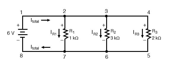
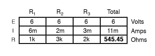
Solving for all values of voltage and current in this circuit:
At this point, we know the value of each branch current and of the total current in the circuit. We know that the total current in a parallel circuit must equal the sum of the branch currents, but there’s more going on in this circuit than just that. Taking a look at the currents at each wire junction point (node) in the circuit, we should be able to see something else:
3.7.3 Currents Entering and Exiting a Node
At each node on the positive “rail” (wire 1-2-3-4) we have current splitting off the main flow to each successive branch resistor. At each node on the negative “rail” (wire 8-7-6-5) we have current merging together to form the main flow from each successive branch resistor. This fact should be fairly obvious if you think of the water pipe circuit analogy with every branch node acting as a “tee” fitting, the water flow splitting or merging with the main piping as it travels from the output of the water pump toward the return reservoir or sump.
If we were to take a closer look at one particular “tee” node, such as node 6, we see that the current entering the node is equal in magnitude to the current exiting the node:
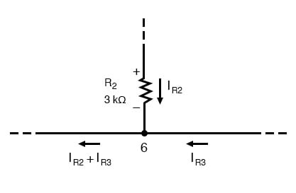
From the top and from the right, we have two currents entering the wire connection labeled as node 6. To the left, we have a single current exiting the node equal in magnitude to the sum of the two currents entering. To refer to the plumbing analogy: so long as there are no leaks in the piping, what flow enters the fitting must also exit the fitting. This holds true for any node (“fitting”), no matter how many flows are entering or exiting. Mathematically, we can express this general relationship as such: [latex]I_{existing}= I_{entering}[/latex]
Kirchhoff’s Current Law
Mr. Kirchhoff decided to express it in a slightly different form (though mathematically equivalent), calling it Kirchhoff’s Current Law (KCL):
[latex]I_{entering}= -I_{existing}=0[/latex]
Summarized in a phrase, Kirchhoff’s Current Law reads as such:
“The algebraic sum of all currents entering and exiting a node must equal zero”
[latex]I_{T} = I_1 + I_2 +... +I_n= 0[/latex]
That is, if we assign a mathematical sign (polarity) to each current, denoting whether they enter (+) or exit (-) a node, we can add them together to arrive at a total of zero, guaranteed.
Taking our example node (number 6), we can determine the magnitude of the current exiting from the left by setting up a KCL equation with that current as the unknown value:
[latex]I_2+I_3+I_{2+3}=0[/latex]
[latex]2mA+ 3mA+I_{2+3} =0[/latex]
[latex]\text{...solving for I...}[/latex]
[latex]I = -2mA-3mA[/latex]
[latex]\pmb{I = -5mA}[/latex]
The negative (-) sign on the value of 5 milliamps tells us that the current is exiting the node, as opposed to the 2 milliamp and 3 milliamp currents, which must both be positive (and therefore entering the node). Whether negative or positive denotes current entering or exiting is entirely arbitrary, so long as they are opposite signs for opposite directions and we stay consistent in our notation, KCL will work.
Together, Kirchhoff’s Voltage and Current Laws are a formidable pair of tools useful in analyzing electric circuits. Their usefulness will become all the more apparent in a later chapter (“Network Analysis”), but suffice it to say that these Laws deserve to be memorized by the electronics student every bit as much as Ohm’s Law.
- Kirchhoff’s Current Law (KCL): “The algebraic sum of all currents entering and exiting a node must equal zero”