
11 CONDUCTORS
11.1 Introduction to Conductance and Conductors
By now you should be well aware of the correlation between electrical conductivity and certain types of materials. Those materials allowing for easy passage of free electrons are called conductors, while those materials impeding the passage of free electrons are called insulators.
Unfortunately, the scientific theories explaining why certain materials conduct and others don’t are quite complex, rooted in quantum mechanical explanations in how electrons are arranged around the nuclei of atoms. Contrary to the well-known “planetary” model of electrons whirling around an atom’s nucleus as well-defined chunks of matter in circular or elliptical orbits, electrons in “orbit” don’t really act like pieces of matter at all. Rather, they exhibit the characteristics of both particle and wave, their behavior constrained by placement within distinct zones around the nucleus referred to as “shells” and “subshells.” Electrons can occupy these zones only in a limited range of energies depending on the particular zone and how occupied that zone is with other electrons. If electrons really did act like tiny planets held in orbit around the nucleus by electrostatic attraction, their actions described by the same laws describing the motions of real planets, there could be no real distinction between conductors and insulators, and chemical bonds between atoms would not exist in the way they do now. It is the discrete, “quantitized” nature of electron energy and placement described by quantum physics that gives these phenomena their regularity.
Excited-state Atom
When an electron is free to assume higher energy states around an atom’s nucleus (due to its placement in a particular “shell”), it may be free to break away from the atom and comprise part of an electric current through the substance.
Ground-state Atom
If the quantum limitations imposed on an electron deny it this freedom, however, the electron is considered to be “bound” and cannot break away (at least not easily) to constitute a current. The former scenario is typical of conducting materials, while the latter is typical of insulating materials.
Some textbooks will tell you that an element’s electrical conductivity is exclusively determined by the number of electrons residing in the atoms’ outer “shell” (called the valence shell), but this is an oversimplification, as any examination of conductivity versus valence electrons in a table of elements will confirm. The true complexity of the situation is further revealed when the conductivity of molecules (collections of atoms bound to one another by electron activity) is considered.
A good example of this is the element carbon, which comprises materials of vastly differing conductivity: graphite and diamond. Graphite is a fair conductor of electricity, while diamond is practically an insulator (stranger yet, it is technically classified as a semiconductor, which in its pure form acts as an insulator, but can conduct under high temperatures and/or the influence of impurities). Both graphite and diamond are composed of the exact same types of atoms: carbon, with 6 protons, 6 neutrons and 6 electrons each. The fundamental difference between graphite and diamond being that graphite molecules are flat groupings of carbon atoms while diamond molecules are tetrahedral (pyramid-shaped) groupings of carbon atoms.
The intentional introduction of impurities into an intrinsic semiconductor for the purpose of altering its electrical, optical, and structural properties is called doping. If atoms of carbon are joined to other types of atoms to form compounds, electrical conductivity becomes altered once again. Silicon carbide, a compound of the elements silicon and carbon, exhibits nonlinear behavior: its electrical resistance decreases with increases in applied voltage! Hydrocarbon compounds (such as the molecules found in oils) tend to be very good insulators. As you can see, a simple count of valence electrons in an atom is a poor indicator of a substance’s electrical conductivity.
All metallic elements are good conductors of electricity, due to the way the atoms bond with each other. The electrons of the atoms comprising a mass of metal are so uninhibited in their allowable energy states that they float freely between the different nuclei in the substance, readily motivated by any electric field. The electrons are so mobile, in fact, that they are sometimes described by scientists as an electron gas, or even an electron sea in which the atomic nuclei rest. This electron mobility accounts for some of the other common properties of metals: good heat conductivity, malleability and ductility (easily formed into different shapes), and a lustrous finish when pure.
Thankfully, the physics behind all this is mostly irrelevant to our purposes here. Suffice it to say that some materials are good conductors, some are poor conductors, and some are in between. For now it is good enough to simply understand that these distinctions are determined by the configuration of the electrons around the constituent atoms of the material.
An important step in getting electricity to do our bidding is to be able to construct paths for current to flow with controlled amounts of resistance. It is also vitally important that we be able to prevent current from flowing where we don’t want it to, by using insulating materials. However, not all conductors are the same, and neither are all insulators. We need to understand some of the characteristics of common conductors and insulators, and be able to apply these characteristics to specific applications.
Almost all conductors possess a certain, measurable resistance (special types of materials called superconductors possess absolutely no electrical resistance, but these are not ordinary materials, and they must be held in special conditions in order to be super conductive). Typically, we assume the resistance of the conductors in a circuit to be zero, and we expect that current passes through them without producing any appreciable voltage drop. In reality, however, there will almost always be a voltage drop along the (normal) conductive pathways of an electric circuit, whether we want a voltage drop to be there or not:

In order to calculate what these voltage drops will be in any particular circuit, we must be able to ascertain the resistance of ordinary wire, knowing the wire size and diameter. Some of the following sections of this chapter will address the details of doing this.
- Electrical conductivity of a material is determined by the configuration of electrons in that materials atoms and molecules (groups of bonded atoms).
- All normal conductors possess resistance to some degree.
- Current flowing through a conductor with (any) resistance will produce some amount of voltage drop across the length of that conductor.
11.2 Conductor Size
It should be common-sense knowledge that liquids flow through large-diameter pipes easier than they do through small-diameter pipes (if you would like a practical illustration, try drinking a liquid through straws of different diameters). The same general principle holds for the flow of electrons through conductors: the broader the cross-sectional area (thickness) of the conductor, the more room for electrons to flow, and consequently, the easier it is for flow to occur (less resistance).
Two Basic Varieties of Electrical Wire: Solid and Stranded
Electrical wire is usually round in cross-section (although there are some unique exceptions to this rule), and comes in two basic varieties: solid and stranded. Solid copper wire is just as it sounds: a single, solid strand of copper the whole length of the wire. Stranded wire is composed of smaller strands of solid copper wire twisted together to form a single, larger conductor. The greatest benefit of stranded wire is its mechanical flexibility, being able to withstand repeated bending and twisting much better than solid copper (which tends to fatigue and break after time).
Wire size can be measured in several ways. We could speak of a wire’s diameter, but since its really the cross-sectional area that matters most regarding the flow of electrons, we are better off designating wire size in terms of area.
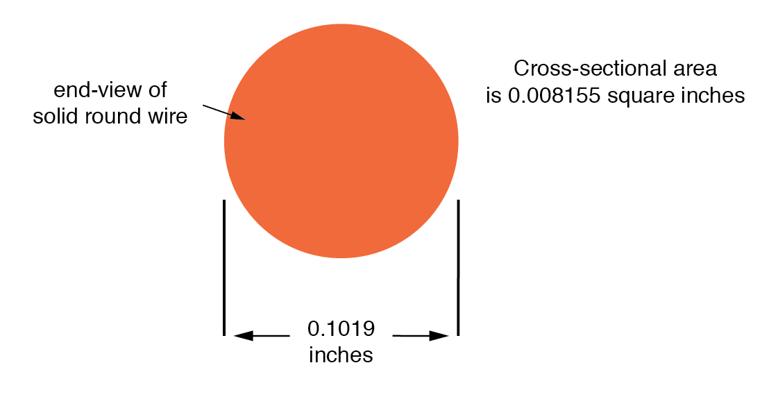
The wire cross-section picture shown above is, of course, not drawn to scale. The diameter is shown as being 0.1019 inches. Calculating the area of the cross-section with the formula Area = πr2, we get an area of 0.008155 square inches:
[latex]A=πr^2[/latex]
[latex]A=(3.1416) (\frac{0.1019 \text{ inches}}{2})^2[/latex]
[latex]A = 0.008155 in^2[/latex]
These are fairly small numbers to work with, so wire sizes are often expressed in measures of thousandths-of-an-inch, or mils. For the illustrated example, we would say that the diameter of the wire was 101.9 mils (0.1019 inch times 1000). We could also, if we wanted, express the area of the wire in the unit of square mils, calculating that value with the same circle-area formula, Area = πr2:
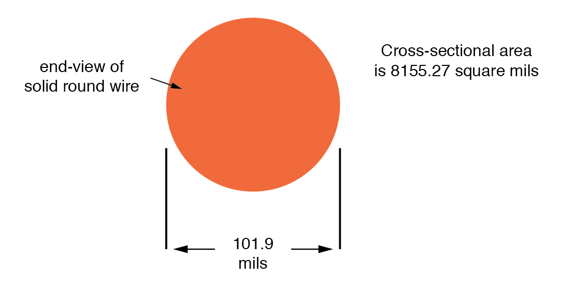
[latex]A=πr^2[/latex]
[latex]=(3.1416) (\frac{101.9 \text{ mils}}{2})^2[/latex]
[latex]= 8155.27 \text{ mils}^2[/latex]
Calculating the Circular-mil Area of a Wire
However, electricians and others frequently concerned with wire size use another unit of area measurement tailored specifically for wire’s circular cross-section. This special unit is called the circular mil (sometimes abbreviated cmil). The sole purpose for having this special unit of measurement is to eliminate the need to invoke the factor π (3.1415927 . . .) in the formula for calculating area, plus the need to figure wire radius when you’ve been given diameter. The formula for calculating the circular-mil area of a circular wire is very simple:
Circular Wire Area Formula
[latex]\tag{11.1} A = d^2[/latex]
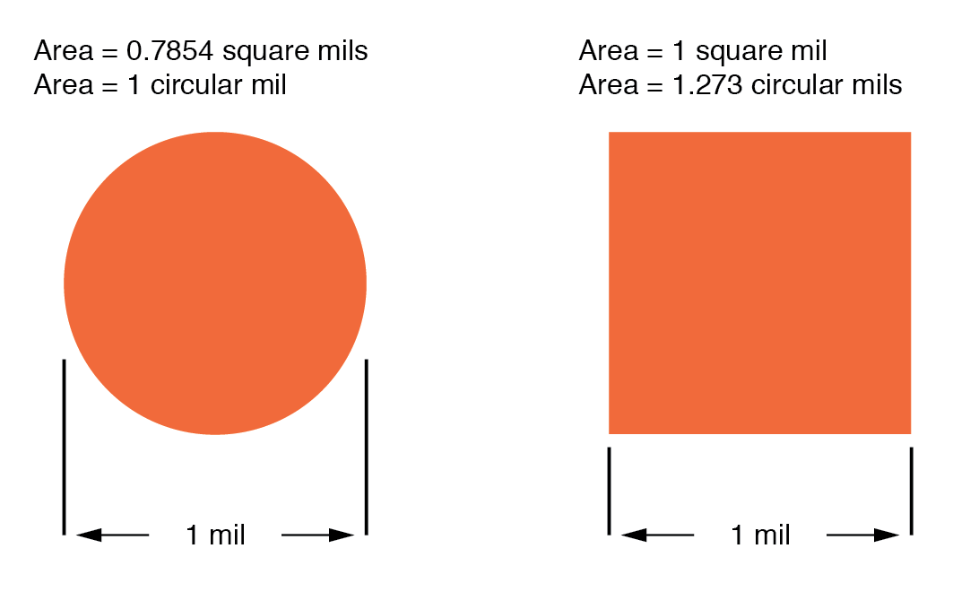
Because this is a unit of area measurement, the mathematical power of 2 is still in effect (doubling the width of a circle will always quadruple its area, no matter what units are used, or if the width of that circle is expressed in terms of radius or diameter). To illustrate the difference between measurements in square mils and measurements in circular mils, I will compare a circle with a square, showing the area of each shape in both unit measures:
And for another size of wire:
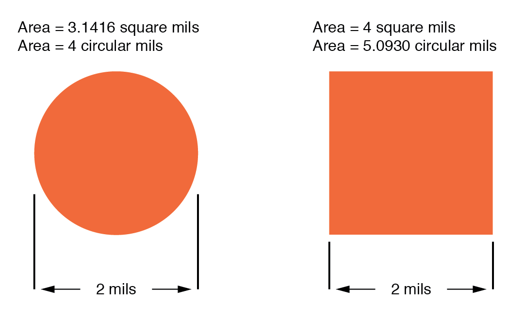
Obviously, the circle of a given diameter has less cross-sectional area than a square of width and height equal to the circle’s diameter: both units of area measurement reflect that. However, it should be clear that the unit of “square mil” is really tailored for the convenient determination of a square’s area, while “circular mil” is tailored for the convenient determination of a circle’s area: the respective formula for each is simpler to work with. It must be understood that both units are valid for measuring the area of a shape, no matter what shape that may be. The conversion between circular mils and square mils is a simple ratio: there are π (3.1415927 . . .) square mils to every 4 circular mils.
Measuring Cross-Sectional Wire Area with Gauge
Another measure of cross-sectional wire area is the gauge. The gauge scale is based on whole numbers rather than fractional or decimal inches. The larger the gauge number, the skinnier the wire; the smaller the gauge number, the fatter the wire. For those acquainted with shotguns, this inversely-proportional measurement scale should sound familiar.
The table at the end of this section equates gauge with inch diameter, circular mils, and square inches for solid wire. The larger sizes of wire reach an end of the common gauge scale (which naturally tops out at a value of 1), and are represented by a series of zeros. “3/0” is another way to represent “000,” and is pronounced “triple-ought.” Again, those acquainted with shotguns should recognize the terminology, strange as it may sound. To make matters even more confusing, there is more than one gauge “standard” in use around the world. For electrical conductor sizing, the American Wire Gauge (AWG), also known as the Brown and Sharpe (B&S) gauge, is the measurement system of choice. In Canada and Great Britain, the British Standard Wire Gauge (SWG) is the legal measurement system for electrical conductors. Other wire gauge systems exist in the world for classifying wire diameter, such as the Stubs steel wire gauge and the Steel Music Wire Gauge (MWG), but these measurement systems apply to non-electrical wire use.
The American Wire Gauge (AWG) measurement system, despite its oddities, was designed with a purpose: for every three steps in the gauge scale, wire area (and weight per unit length) approximately doubles. This is a handy rule to remember when making rough wire size estimations!
For very large wire sizes (fatter than 4/0), the wire gauge system is typically abandoned for cross-sectional area measurement in thousands of circular mils (MCM), borrowing the old Roman numeral “M” to denote a multiple of “thousand” in front of “CM” for “circular mils.” The following table of wire sizes does not show any sizes bigger than 4/0 gauge, because solid copper wire becomes impractical to handle at those sizes. Stranded wire construction is favored, instead.
Wire Table For Solid, Round Copper Conductors
| Size | Diameter | Cross-sectional area | Weight | |
|---|---|---|---|---|
| AWG | Inches | cir. mils | sq. inches | lb/1000 ft |
| 4/0 | 0.4600 | 211,600 | 0.1662 | 640.5 |
| 3/0 | 0.4096 | 167,800 | 0.1318 | 507.9 |
| 2/0 | 0.3648 | 133,100 | 0.1045 | 402.8 |
| 1/0 | 0.3249 | 105,500 | 0.08289 | 319.5 |
| 1 | 0.2893 | 83,690 | 0.06573 | 253.5 |
| 2 | 0.2576 | 66,370 | 0.05213 | 200.9 |
| 3 | 0.2294 | 52,630 | 0.04134 | 159.3 |
| 4 | 0.2043 | 41,740 | 0.03278 | 126.4 |
| 5 | 0.1819 | 33,100 | 0.02600 | 100.2 |
| 6 | 0.1620 | 26,250 | 0.02062 | 79.46 |
| 7 | 0.1443 | 20,820 | 0.01635 | 63.02 |
| 8 | 0.1285 | 16,510 | 0.01297 | 49.97 |
| 9 | 0.1144 | 13,090 | 0.01028 | 39.63 |
| 10 | 0.1019 | 10,380 | 0.008155 | 31.43 |
| 11 | 0.09074 | 8,234 | 0.006467 | 24.92 |
| 12 | 0.08081 | 6,530 | 0.005129 | 19.77 |
| 13 | 0.07196 | 5,178 | 0.004067 | 15.68 |
| 14 | 0.06408 | 4,107 | 0.003225 | 12.43 |
| 15 | 0.05707 | 3,257 | 0.002558 | 9.858 |
| 16 | 0.05082 | 2,583 | 0.002028 | 7.818 |
| 17 | 0.04526 | 2,048 | 0.001609 | 6.200 |
| 18 | 0.04030 | 1,624 | 0.001276 | 4.917 |
| 19 | 0.03589 | 1,288 | 0.001012 | 3.899 |
| 20 | 0.03196 | 1,022 | 0.0008023 | 3.092 |
| 21 | 0.02846 | 810.1 | 0.0006363 | 2.452 |
| 22 | 0.02535 | 642.5 | 0.0005046 | 1.945 |
| 23 | 0.02257 | 509.5 | 0.0004001 | 1.542 |
| 24 | 0.02010 | 404.0 | 0.0003173 | 1.233 |
| 25 | 0.01790 | 320.4 | 0.0002517 | 0.9699 |
| 26 | 0.01594 | 254.1 | 0.0001996 | 0.7692 |
| 27 | 0.01420 | 201.5 | 0.0001583 | 0.6100 |
| 28 | 0.01264 | 159.8 | 0.0001255 | 0.4837 |
| 29 | 0.01126 | 126.7 | 0.00009954 | 0.3836 |
| 30 | 0.01003 | 100.5 | 0.00007894 | 0.3042 |
| 31 | 0.008928 | 79.70 | 0.00006260 | 0.2413 |
| 32 | 0.007950 | 63.21 | 0.00004964 | 0.1913 |
| 33 | 0.007080 | 50.13 | 0.00003937 | 0.1517 |
| 34 | 0.006305 | 39.75 | 0.00003122 | 0.1203 |
| 35 | 0.005615 | 31.52 | 0.00002476 | 0.09542 |
| 36 | 0.005000 | 25.00 | 0.00001963 | 0.07567 |
| 37 | 0.004453 | 19.83 | 0.00001557 | 0.06001 |
| 38 | 0.003965 | 15.72 | 0.00001235 | 0.04759 |
| 39 | 0.003531 | 12.47 | 0.000009793 | 0.03774 |
| 40 | 0.003145 | 9.888 | 0.000007766 | 0.02993 |
| 41 | 0.002800 | 7.842 | 0.000006159 | 0.02374 |
| 42 | 0.002494 | 6.219 | 0.000004884 | 0.01882 |
| 43 | 0.002221 | 4.932 | 0.000003873 | 0.01493 |
For some high-current applications, conductor sizes beyond the practical size limit of round wire are required. In these instances, thick bars of solid metal called busbars are used as conductors. Busbars are usually made of copper or aluminum, and are most often uninsulated. They are physically supported away from whatever framework or structure is holding them by insulator standoff mounts. Although a square or rectangular cross-section is very common for busbar shape, other shapes are used as well. Cross-sectional area for busbars is typically rated in terms of circular mils (even for square and rectangular bars!), most likely for the convenience of being able to directly equate busbar size with round wire.
- Current flows through large-diameter wires easier than small-diameter wires, due to the greater cross-sectional area they have in which to move.
- Rather than measure small wire sizes in inches, the unit of “mil” (1/1000 of an inch) is often employed.
- The cross-sectional area of a wire can be expressed in terms of square units (square inches or square mils), circular mils, or “gauge” scale.
- Calculating square-unit wire area for a circular wire involves the circle area formula:
- A = πr2 (square units)
- Calculating circular-mil wire area for a circular wire is much simpler, due to the fact that the unit of “circular mil” was sized just for this purpose: to eliminate the “pi” and the d/2 (radius) factors in the formula.
- A = d2 (circular units)
- There are π (3.1416) square mils for every 4 circular mils.
- The gauge system of wire sizing is based on whole numbers, larger numbers representing smaller-area wires and vice versa. Wires thicker than 1 gauge are represented by zeros: 0, 00, 000, and 0000 (spoken “single-ought,” “double-ought,” “triple-ought,” and “quadruple-ought.”
- Very large wire sizes are rated in thousands of circular mils (MCM’s), typical for busbars and wire sizes beyond 4/0.
- Busbars are solid bars of copper or aluminum used in high-current circuit construction. Connections made to busbars are usually welded or bolted, and the busbars are often bare (uninsulated), supported away from metal frames through the use of insulating standoffs.
11.3 Conductor Ampacity
The smaller the cross-sectional area of any given wire, the greater the resistance for any given length, all other factors being equal. A wire with greater resistance will dissipate a greater amount of heat energy for any given amount of current, the power being equal to P=I2R.
Dissipated power due to a conductor’s resistance manifests itself in the form of heat, and excessive heat can be damaging to a wire (not to mention objects near the wire), especially considering the fact that most wires are insulated with a plastic or rubber coating, which can melt and burn. Thin wires will, therefore, tolerate less current than thick wires, all other factors being equal. A conductor’s current-carrying limit is known as its ampacity.
Primarily for reasons of safety, certain standards for electrical wiring have been established within the United States, and are specified in the National Electrical Code (NEC). Typical NEC wire ampacity tables will show allowable maximum currents for different sizes and applications of wire. Though the melting point of copper theoretically imposes a limit on wire ampacity, the materials commonly employed for insulating conductors melt at temperatures far below the melting point of copper, and so practical ampacity ratings are based on the thermal limits of the insulation. Voltage dropped as a result of excessive wire resistance is also a factor in sizing conductors for their use in circuits, but this consideration is better assessed through more complex means (which we will cover in this chapter). A table derived from an NEC listing is shown for example:
Table 11.2 Copper Conductor Ampacities, in Free Air at 30 Degrees C
| Insulation: | RUW, T | THW, THWN | FEP, FEPB |
|---|---|---|---|
| Type: | TW | RUH | THHN, XHHW |
| Size | Current Rating | Current Rating | Current Rating |
|---|---|---|---|
| AWG | @ 60 degrees C | @ 75 degrees C | @ 90 degrees C |
| 20 | *9 | – | *12.5 |
| 19 | *13 | – | 18 |
| 16 | *18 | – | 24 |
| 14 | 25 | 30 | 35 |
| 12 | 30 | 35 | 40 |
| 10 | 40 | 50 | 55 |
| 8 | 60 | 70 | 80 |
| 6 | 80 | 95 | 105 |
| 4 | 105 | 125 | 140 |
| 2 | 140 | 170 | 190 |
| 1 | 165 | 195 | 220 |
| 1/0 | 195 | 230 | 260 |
| 2/0 | 225 | 265 | 300 |
| 3/0 | 260 | 310 | 350 |
| 4/0 | 300 | 360 | 405 |
* = estimated values; normally, these small wire sizes are not manufactured with these insulation types
Notice the substantial ampacity differences between same-size wires with different types of insulation. This is due, again, to the thermal limits (60°, 75°, 90°) of each type of insulation material.
These ampacity ratings are given for copper conductors in “free air” (maximum typical air circulation), as opposed to wires placed in conduit or wire trays. As you will notice, the table fails to specify ampacities for small wire sizes. This is because the NEC concerns itself primarily with power wiring (large currents, big wires) rather than with wires common to low-current electronic work.
There is meaning in the letter sequences used to identify conductor types, and these letters usually refer to properties of the conductor’s insulating layer(s). Some of these letters symbolize individual properties of the wire while others are simply abbreviations. For example, the letter “T” by itself means “thermoplastic” as an insulation material, as in “TW” or “THHN.” However, the three-letter combination “MTW” is an abbreviation for Machine Tool Wire, a type of wire whose insulation is made to be flexible for use in machines experiencing significant motion or vibration.
Insulation Material
- C = Cotton
- FEP = Fluorinated Ethylene Propylene
- MI = Mineral (magnesium oxide)
- PFA = Perfluoroalkoxy
- R = Rubber (sometimes Neoprene)
- S = Silicone “rubber”
- SA = Silicone-asbestos
- T = Thermoplastic
- TA = Thermoplastic-asbestos
- TFE = Polytetrafluoroethylene (“Teflon”)
- X = Cross-linked synthetic polymer
- Z = Modified ethylene tetrafluoroethylene
Heat Rating
- H = 75 degrees Celsius
- HH = 90 degrees Celsius
Outer Covering (“Jacket”)
- N = Nylon
Special Service Conditions
- U = Underground
- W = Wet
- -2 = 90 degrees Celsius and wet
Therefore, a “THWN” conductor has Thermoplastic insulation, is Heat resistant to 75° Celsius, is rated for Wet conditions, and comes with a Nylon outer jacketing.
Letter codes like these are only used for general-purpose wires such as those used in households and businesses. For high-power applications and/or severe service conditions, the complexity of conductor technology defies classification according to a few letter codes. Overhead power line conductors are typically bare metal, suspended from towers by glass, porcelain, or ceramic mounts known as insulators. Even so, the actual construction of the wire to withstand physical forces both static (dead weight) and dynamic (wind) loading can be complex, with multiple layers and different types of metals wound together to form a single conductor. Large, underground power conductors are sometimes insulated by paper, then enclosed in a steel pipe filled with pressurized nitrogen or oil to prevent water intrusion. Such conductors require support equipment to maintain fluid pressure throughout the pipe.
Other insulating materials find use in small-scale applications. For instance, the small-diameter wire used to make electromagnets (coils producing a magnetic field from the flow of electrons) are often insulated with a thin layer of enamel. The enamel is an excellent insulating material and is very thin, allowing many “turns” of wire to be wound in a small space.
- Wire resistance creates heat in operating circuits. This heat is a potential fire ignition hazard.
- Skinny wires have a lower allowable current (“ampacity”) than fat wires, due to their greater resistance per unit length, and consequently greater heat generation per unit current.
- The National Electrical Code (NEC) specifies ampacities for power wiring based on allowable insulation temperature and wire application.
11.4 Specific Resistance
Designing Wire Resistance
Conductor ampacity rating is a crude assessment of resistance based on the potential for current to create a fire hazard. However, we may come across situations where the voltage drop created by wire resistance in a circuit poses concerns other than fire avoidance. For instance, we may be designing a circuit where voltage across a component is critical, and must not fall below a certain limit. If this is the case, the voltage drops resulting from wire resistance may cause an engineering problem while being well within safe (fire) limits of ampacity:
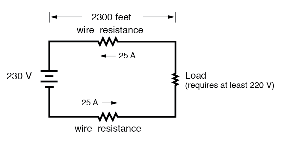
If the load in the above circuit will not tolerate less than 220 volts, given a source voltage of 230 volts, then we’d better be sure that the wiring doesn’t drop more than 10 volts along the way. Counting both the supply and return conductors of this circuit, this leaves a maximum tolerable drop of 5 volts along the length of each wire. Using Ohm’s Law (R=E/I), we can determine the maximum allowable resistance for each piece of wire:
[latex]R = \frac{E}{I}[/latex]
[latex]= \frac{5V}{25A}[/latex]
[latex]R= 0.2Ω[/latex]
We know that the wire length is 2300 feet for each piece of wire, but how do we determine the amount of resistance for a specific size and length of wire? To do that, we need another formula:
This formula relates the resistance of a conductor with its specific resistance (the Greek letter “rho” (ρ), which looks similar to a lower-case letter “p”), its length (“l”), and its cross-sectional area (“A”). Notice that with the length variable on the top of the fraction, the resistance value increases as the length increases (analogy: it is more difficult to force liquid through a long pipe than a short one), and decreases as cross-sectional area increases (analogy: liquid flows easier through a fat pipe than through a skinny one). Specific resistance is a constant for the type of conductor material being calculated.
The specific resistances of several conductive materials can be found in the following table. We find copper near the bottom of the table, second only to silver in having low specific resistance (good conductivity):
Table 11.3 Specific Resistance at 20 Degrees Celsius
| Material | Element/Alloy | (ohm-cmil/ft) | (microohm-cm) |
|---|---|---|---|
| Nichrome | Alloy | 675 | 112.2 |
| Nichrome V | Alloy | 650 | 108.1 |
| Manganin | Alloy | 290 | 48.21 |
| Constantan | Alloy | 272.97 | 45.38 |
| Steel* | Alloy | 100 | 16.62 |
| Platinum | Element | 63.16 | 10.5 |
| Iron | Element | 57.81 | 9.61 |
| Nickel | Element | 41.69 | 6.93 |
| Zinc | Element | 35.49 | 5.90 |
| Molybdenum | Element | 32.12 | 5.34 |
| Tungsten | Element | 31.76 | 5.28 |
| Aluminum | Element | 15.94 | 2.650 |
| Gold | Element | 13.32 | 2.214 |
| Copper | Element | 10.09 | 1.678 |
| Silver | Element | 9.546 | 1.587 |
* = Steel alloy at 99.5 percent iron, 0.5 percent carbon
Notice that the figures for specific resistance in the above table are given in the very strange unit of “ohms-cmil/ft” (Ω-cmil/ft), This unit indicates what units we are expected to use in the resistance formula ([latex]\text{R}= \rho \ell / \text{A}[/latex]). In this case, these figures for specific resistance are intended to be used when length is measured in feet and cross-sectional area is measured in circular mils.
The metric unit for specific resistance is the ohm-meter (Ω-m), or ohm-centimeter (Ω-cm), with 1.66243 x 10⁻⁹ Ω-meters per Ω-cmil/ft (1.66243 x 10⁻⁷ Ω-cm per Ω-cmil/ft). In the Ω-cm column of the table, the figures are actually scaled as µΩ-cm due to their very small magnitudes. For example, iron is listed as 9.61 µΩ-cm, which could be represented as 9.61 x 10⁻⁶ Ω-cm.
When using the unit of Ω-meter for specific resistance in the [latex]\text{R}= \rho \ell / \text{A}[/latex] formula, the length needs to be in meters and the area in square meters. When using the unit of Ω-centimeter (Ω-cm) in the same formula, the length needs to be in centimeters and the area in square centimeters.
All these units for specific resistance are valid for any material (Ω-cmil/ft, Ω-m, or Ω-cm). One might prefer to use Ω-cmil/ft, however, when dealing with round wire where the cross-sectional area is already known in circular mils. Conversely, when dealing with odd-shaped busbar or custom busbar cut out of metal stock, where only the linear dimensions of length, width, and height are known, the specific resistance units of Ω-meter or Ω-cm may be more appropriate.
Going back to our example circuit, we were looking for wire that had 0.2 Ω or less of resistance over a length of 2300 feet. Assuming that we’re going to use copper wire (the most common type of electrical wire manufactured), we can set up our formula as such:
[latex]R= ρ\frac{e}{A}[/latex]
Solving for area (A):
[latex]A= ρ\frac{e}{R}[/latex]
[latex]= (10.09Ω-cmil/ft)(\frac{2300feet}{0.2Ω})[/latex]
[latex]= 116,035cmils[/latex]
Algebraically solving for A, we get a value of 116,035 circular mils. Referencing our solid wire size table, we find that “double-ought” (2/0) wire with 133,100 cmils is adequate, whereas the next lower size, “single-ought” (1/0), at 105,500 cmils is too small. Bear in mind that our circuit current is a modest 25 amps. According to our ampacity table for copper wire in free air, 14 gauge wire would have sufficed (as far as not starting a fire is concerned). However, from the standpoint of voltage drop, 14 gauge wire would have been very unacceptable.
Just for fun, let’s see what 14 gauge wire would have done to our power circuit’s performance. Looking at our wire size table, we find that 14 gauge wire has a cross-sectional area of 4,107 circular mils. If we’re still using copper as a wire material (a good choice, unless we’re really rich and can afford 4600 feet of 14 gauge silver wire!), then our specific resistance will still be 10.09 Ω-cmil/ft:
[latex]R= ρ\frac{e}{A}[/latex]
[latex]= (10.09Ω-cmil/ft)(\frac{2300feet}{4107})[/latex]
[latex]= 5.651Ω[/latex]
Remember that this is 5.651 Ω per 2300 feet of 14-gauge copper wire, and that we have two runs of 2300 feet in the entire circuit, so each wire piece in the circuit has 5.651 Ω of resistance:
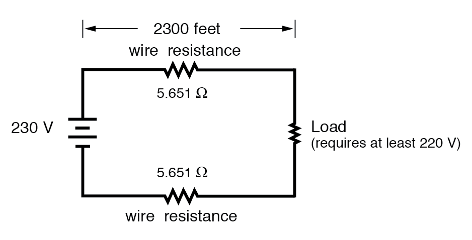
Our total circuit wire resistance is 2 times 5.651, or 11.301 Ω. Unfortunately, this is far too much resistance to allow 25 amps of current with a source voltage of 230 volts. Even if our load resistance was 0 Ω, our wiring resistance of 11.301 Ω would restrict the circuit current to a mere 20.352 amps! As you can see, a “small” amount of wire resistance can make a big difference in circuit performance, especially in power circuits where the currents are much higher than typically encountered in electronic circuits.
Let’s do an example resistance problem for a piece of custom-cut busbar. Suppose we have a piece of solid aluminum bar, 4 centimeters wide by 3 centimeters tall by 125 centimeters long, and we wish to figure the end-to-end resistance along the long dimension (125 cm). First, we would need to determine the cross-sectional area of the bar:
[latex]Area = {width} ×{Height}[/latex]
[latex]A = {4cm} ×{3cm}[/latex]
[latex]= 12cm^2[/latex]
We also need to know the specific resistance of aluminum, in the unit proper for this application (Ω-cm). From our table of specific resistances, we see that this is 2.65 x 10⁻⁶ Ω-cm. Setting up our R=ρl/A formula, we have:
[latex]R= ρ\frac{e}{A}[/latex]
[latex]= (2.65 × 10^-6 Ω-cm)(\frac{125cm}{12cm^2})[/latex]
[latex]= 27.604μΩ[/latex]
As you can see, the sheer thickness of a busbar makes for very low resistances compared to that of standard wire sizes, even when using a material with a greater specific resistance.
The procedure for determining busbar resistance is not fundamentally different than for determining round wire resistance. We just need to make sure that cross-sectional area is calculated properly and that all the units correspond to each other as they should.
- Conductor resistance increases with increased length and decreases with increased cross-sectional area, all other factors being equal.
- Specific Resistance (”ρ”) is a property of any conductive material, a figure used to determine the end-to-end resistance of a conductor given length and area in this formula: R = ρl/A
- Specific resistance for materials are given in units of Ω-cmil/ft or Ω-meters (metric). Conversion factor between these two units is 1.66243 x 10⁻⁹ Ω-meters per Ω-cmil/ft, or 1.66243 x 10⁻⁷ Ω-cm per Ω-cmil/ft.
- If wiring voltage drop in a circuit is critical, exact resistance calculations for the wires must be made before wire size is chosen.
11.5 Temperature Coefficient of Resistance
You might have noticed on the table for specific resistances that all figures were specified at a temperature of 20° Celsius. If you suspected that this meant specific resistance of a material may change with temperature, you were right!
Resistance values for conductors at any temperature other than the standard temperature (usually specified at 20 Celsius) on the specific resistance table must be determined through yet another formula:
[latex]R = R_{ref}[1+α(T-T_{ref})] \tag{11.3}[/latex]
Where,
[latex]R = \text{Conductance resistance at temperature "T"}[/latex]
[latex]R_{ref} = \text{Conductance resistance at reference temperature}[/latex]
[latex]T_{ref} =\text{ usually }20°C\text{, but sometimes }0°C[/latex]
[latex]α = \text{Temperature coefficient of resistance for conductor material}[/latex]
[latex]\text{T = Conductor temperature in degree Celsius}[/latex]
[latex]T_{ref} =\text{Reference temperature that α is specified at for the conductor}[/latex]
The “alpha” (α) constant is known as the temperature coefficient of resistance and symbolizes the resistance change factor per degree of temperature change. Just as all materials have a certain specific resistance (at 20° C), they also change resistance according to temperature by certain amounts. For pure metals, this coefficient is a positive number, meaning that resistance increases with increasing temperature. For the elements carbon, silicon, and germanium, this coefficient is a negative number, meaning that resistance decreases with increasing temperature. For some metal alloys, the temperature coefficient of resistance is very close to zero, meaning that the resistance hardly changes at all with variations in temperature (a good property if you want to build a precision resistor out of metal wire!). The following table gives the temperature coefficients of resistance for several common metals, both pure and alloy:
Table 11.4 Temperature Coefficients of Resistance at 20 Degrees Celsius
| Material | Element/Alloy | “alpha” per degree Celsius |
|---|---|---|
| Nickel | Element | 0.005866 |
| Iron | Element | 0.005671 |
| Molybdenum | Element | 0.004579 |
| Tungsten | Element | 0.004403 |
| Aluminum | Element | 0.004308 |
| Copper | Element | 0.004041 |
| Silver | Element | 0.003819 |
| Platinum | Element | 0.003729 |
| Gold | Element | 0.003715 |
| Zinc | Element | 0.003847 |
| Steel* | Alloy | 0.003 |
| Nichrome | Alloy | 0.00017 |
| Nichrome V | Alloy | 0.00013 |
| Manganin | Alloy | +/- 0.000015 |
| Constantan | Alloy | -0.000074 |
* = Steel alloy at 99.5 percent iron, 0.5 percent carbon tys
Let’s take a look at an example circuit to see how temperature can affect wire resistance, and consequently circuit performance:
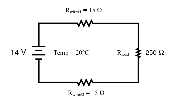
This circuit has a total wire resistance (wire 1 + wire 2) of 30 Ω at standard temperature. Setting up a table of voltage, current, and resistance values we get:
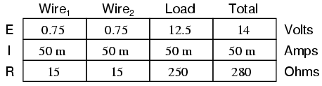
At 20° Celsius, we get 12.5 volts across the load and a total of 1.5 volts (0.75 + 0.75) dropped across the wire resistance. If the temperature were to rise to 35° Celsius, we could easily determine the change of resistance for each piece of wire. Assuming the use of copper wire (α = 0.004041) we get:
[latex]R = R_{ref}[1+α(T-T_{ref})][/latex]
[latex]= (15Ω)[1+0.004041(35°-20°)][/latex]
[latex]= 15.909Ω[/latex]
Recalculating our circuit values, we see what changes this increase in temperature will bring:
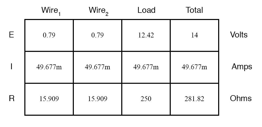
As you can see, voltage across the load went down (from 12.5 volts to 12.42 volts) and voltage drop across the wires went up (from 0.75 volts to 0.79 volts) as a result of the temperature increasing. Though the changes may seem small, they can be significant for power lines stretching miles between power plants and substations, substations and loads. In fact, power utility companies often have to take line resistance changes resulting from seasonal temperature variations into account when calculating allowable system loading.
- Most conductive materials change specific resistance with changes in temperature. This is why figures of specific resistance are always specified at a standard temperature (usually 20° or 25° Celsius).
- The resistance-change factor per degree Celsius of temperature change is called the temperature coefficient of resistance. This factor is represented by the Greek lower-case letter “alpha” (α).
- A positive coefficient for a material means that its resistance increases with an increase in temperature. Pure metals typically have positive temperature coefficients of resistance. Coefficients approaching zero can be obtained by alloying certain metals.
- A negative coefficient for a material means that its resistance decreases with an increase in temperature. Semiconductor materials (carbon, silicon, germanium) typically have negative temperature coefficients of resistance.
11.6 Insulator Breakdown Voltage
The atoms in insulating materials have very tightly-bound electrons, resisting free electron flow very well. However, insulators cannot resist indefinite amounts of voltage. With enough voltage applied, any insulating material will eventually succumb to the electrical “pressure,” and then current flow will occur. However, unlike the situation with conductors where current is in linear proportion to applied voltage (given a fixed resistance), current through an insulator is quite nonlinear: for voltages below a certain threshold, virtually no current will flow, but if the applied voltage exceeds that threshold voltage (known as the breakdown voltage or dielectric strength), there will be a rush of current.
Dielectric strength is the voltage required to cause dielectric breakdown, that is, to force current through an insulating material. After dielectric breakdown, the material may or may not behave as an insulator any more, the molecular structure having been altered by the breach. There is usually a localized “puncture” of the insulating medium where the current flowed during breakdown.
The thickness of an insulating material plays a role in determining its breakdown voltage. Specific dielectric strength is sometimes listed in terms of volts per mil (1/1000 of an inch), or kilovolts per inch (the two units are equivalent), but in practice it has been found that the relationship between breakdown voltage and thickness is not exactly linear. An insulator three times as thick has a dielectric strength slightly less than 3 times as much. However, for rough estimation use, volt-per-thickness ratings are fine.
| Material* | Dielectric strength (kV/inch) |
|---|---|
| Vacuum | 20 |
| Air | 20 to 75 |
| Porcelain | 40 to 200 |
| Paraffin Wax | 200 to 300 |
| Transformer Oil | 400 |
| Bakelite | 300 to 550 |
| Rubber | 450 to 700 |
| Shellac | 900 |
| Paper | 1250 |
| Teflon | 1500 |
| Glass | 2000 to 3000 |
| Mica | 5000 |
* = Materials listed are specially prepared for electrical use.
- With a high enough applied voltage, electrons can be freed from the atoms of insulating materials, resulting in current through that material.
- The minimum voltage required to “break” an insulator by forcing current through it is called the breakdown voltage or dielectric strength.
- The thicker a piece of insulating material, the higher the breakdown voltage, all other factors being equal.
- Specific dielectric strength is typically rated in one of two equivalent units: volts per mil, or kilovolts per inch.