
6 REACTIVE POWER
6.1 AC Resistor Circuits
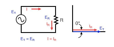
If we were to plot the current and voltage for a very simple AC circuit consisting of a source and a resistor (figure above), it would look something like this: (figure below)
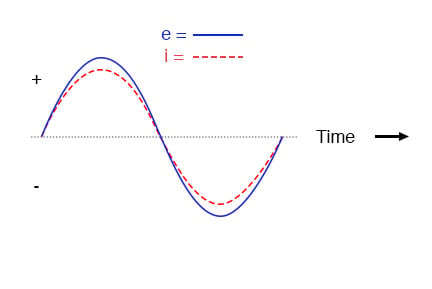
Because the resistor simply and directly resists the flow of current at all periods of time, the waveform for the voltage drop across the resistor is exactly in phase with the waveform for the current through it. We can look at any point in time along the horizontal axis of the plot and compare those values of current and voltage with each other (any “snapshot” look at the values of a wave are referred to as instantaneous values, meaning the values at that instant in time). When the instantaneous value for the current is zero, the instantaneous voltage across the resistor is also zero. Likewise, at the moment in time where the current through the resistor is at its positive peak, the voltage across the resistor is also at its positive peak, and so on. At any given point in time along the waves, Ohm’s Law holds true for the instantaneous values of voltage and current.
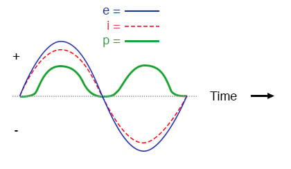
We can also calculate the power dissipated by this resistor, and plot those values on the same graph: (figure below)
6.2 AC Inductor Circuits
Resistors vs. Inductors
Inductors do not behave the same way as resistors do. Whereas resistors simply oppose the flow of current through them (by dropping a voltage directly proportional to the current), inductors oppose changes in current through them, by dropping a voltage directly proportional to the rate of change of current. In accordance with Lenz’s Law, this induced voltage is always of such a polarity as to try to maintain current at its present value. That is, if the current is increasing in magnitude, the induced voltage will “push against” the current flow; if the current is decreasing, the polarity will reverse and “push with” the current to oppose the decrease. This opposition to current change is called reactance, rather than resistance. Expressed mathematically, the relationship between the voltage dropped across the inductor and rate of current change through the inductor is as such:
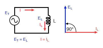
Alternating Current in a Simple Inductive Circuit
The expression di/dt is one from calculus, meaning the rate of change of instantaneous current (i) over time, in amps per second. The inductance (L) is in Henrys, and the instantaneous voltage (e), of course, is in volts. Sometimes you will find the rate of instantaneous voltage expressed as “v” instead of “e” (v = L di/dt), but it means the exact same thing. To show what happens with alternating current, let’s analyze a simple inductor circuit:
If we were to plot the current and voltage for this very simple circuit, it would look something like this:
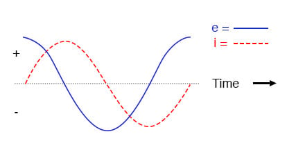
Remember, the voltage dropped across an inductor is a reaction against the change in current through it. Therefore, the instantaneous voltage is zero whenever the instantaneous current is at a peak (zero change, or level slope, on the current sine wave), and the instantaneous voltage is at a peak wherever the instantaneous current is at maximum change (the points of steepest slope on the current wave, where it crosses the zero line). This results in a voltage wave that is 90° out of phase with the current wave. Looking at the graph, the voltage wave seems to have a “head start” on the current wave; the voltage “leads” the current and the current “lags” behind the voltage.
Things get even more interesting when we plot the power for this circuit:
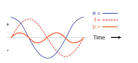
Because instantaneous power is the product of the instantaneous voltage and the instantaneous current (p=ie), the power equals zero whenever the instantaneous current or voltage is zero. Whenever the instantaneous current and voltage are both positive (above the line), the power is positive. As with the resistor example, the power is also positive when the instantaneous current and voltage are both negative (below the line). However, because the current and voltage waves are 90° out of phase, there are times when one is positive while the other is negative, resulting in equally frequent occurrences of negative instantaneous power.
What is Negative Power?
But what does negative power mean? It means that the inductor is releasing power back to the circuit, while a positive power means that it is absorbing power from the circuit. Since the positive and negative power cycles are equal in magnitude and duration over time, the inductor releases just as much power back to the circuit as it absorbs over the span of a complete cycle. What this means in a practical sense is that the reactance of an inductor dissipates net energy of zero, quite unlike the resistance of a resistor, which dissipates energy in the form of heat. Mind you, this is for perfect inductors only, which have no wire resistance.
Reactance vs. Resistance
An inductor’s opposition to change in current translates to an opposition to alternating current in general, which is by definition always changing in instantaneous magnitude and direction. This opposition to alternating current is similar to resistance but different in that it always results in a phase shift between current and voltage, and it dissipates zero power. Because of the differences, it has a different name: reactance. Reactance to AC is expressed in ohms, just like resistance is, except that its mathematical symbol is X instead of R. To be specific, reactance associated with an inductor is usually symbolized by the capital letter X with a letter L as a subscript, like this: XL.
Since inductors drop voltage in proportion to the rate of current change, they will drop more voltage for faster-changing currents, and less voltage for slower-changing currents. What this means is that reactance in ohms for any inductor is directly proportional to the frequency of the alternating current. The exact formula for determining reactance is as follows:
If we expose a 10 mH inductor to frequencies of 60, 120, and 2500 Hz, it will manifest the reactances in the table below.
Reactance of a 10 mH inductor:
| Frequency (Hertz) | Reactance (Ohms) |
| 60 | 3.7699 |
| 120 | 7.5398 |
| 2500 | 157.0796 |
In the reactance equation, the term “2πf” (everything on the right-hand side except the L) has a special meaning unto itself. It is the number of radians per second that the alternating current is “rotating” at, if you imagine one cycle of AC to represent a full circle’s rotation. A radian is a unit of angular measurement: there are 2π radians in one full circle, just as there are 360° in a full circle. If the alternator producing the AC is a double-pole unit, it will produce one cycle for every full turn of shaft rotation, which is every 2π radians, or 360°. If this constant of 2π is multiplied by frequency in Hertz (cycles per second), the result will be a figure in radians per second, known as the angular velocity of the AC system.
Angular Velocity in AC Systems
Angular velocity may be represented by the expression 2πf, or it may be represented by its own symbol, the lowercase Greek letter omega, which appears similar to our Roman lower-case “w”: ω. Thus, the reactance formula XL = 2πfL could also be written as XL = ωL.
It must be understood that this “angular velocity” is an expression of how rapidly the AC waveforms are cycling, a full-cycle being equal to 2π radians. It is not necessarily representative of the actual shaft speed of the alternator producing the AC. If the alternator has more than two poles, the angular velocity will be a multiple of the shaft speed. For this reason, ω is sometimes expressed in units of electrical radians per second rather than (plain) radians per second, so as to distinguish it from mechanical motion.
Any way we express the angular velocity of the system, it is apparent that it is directly proportional to reactance in an inductor. As the frequency (or alternator shaft speed) is increased in an AC system, an inductor will offer greater opposition to the passage of current, and vice versa. Alternating current in a simple inductive circuit is equal to the voltage (in volts) divided by the inductive reactance (in ohms), just as either alternating or direct current in a simple resistive circuit is equal to the voltage (in volts) divided by the resistance (in ohms). An example circuit is shown here:
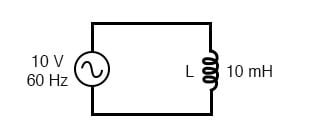
(Inductive reactance of 10 mH inductor at 60Hz)
[latex]X_L =3.7600Ω[/latex]
[latex]I_{X_{L}} = \frac{E}{X}[/latex]
[latex]= \frac{10V}{3.7600Ω}[/latex]
[latex]\mathbf{= 2.6526A}[/latex]
Phase Angles
However, we need to keep in mind that voltage and current are not in phase here. As was shown earlier, the voltage has a phase shift of +90° with respect to the current. If we represent these phase angles of voltage and current mathematically in the form of complex numbers, we find that an inductor’s opposition to current has a phase angle, too:
[latex]\text{Opposition }= \frac{\text{Voltage}}{\text{Current}}[/latex]
[latex]\text{Opposition }= \frac{10 V \angle \text{90°}}{2.6526A \angle \text{90°}}[/latex]
[latex]\begin{align} \text{Opposition } = & 3.7699 \Omega \angle \text{90°} \\ \text { or } & 0 + j3.7699 \Omega \end{align}[/latex]
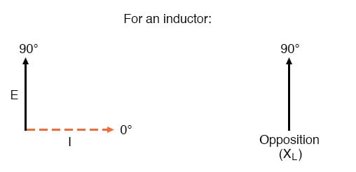
Mathematically, we say that the phase angle of an inductor’s opposition to current is 90°, meaning that an inductor’s opposition to current is a positive imaginary quantity. This phase angle of reactive opposition to current becomes critically important in circuit analysis, especially for complex AC circuits where reactance and resistance interact. It will prove beneficial to represent any component’s opposition to current in terms of complex numbers rather than scalar quantities of resistance and reactance.
- Inductive reactance is the opposition that an inductor offers to alternating current due to its phase-shifted storage and release of energy in its magnetic field. Reactance is symbolized by the capital letter “X” and is measured in ohms just like resistance (R).
- Inductive reactance can be calculated using this formula: XL = 2πfL
- The angular velocity of an AC circuit is another way of expressing its frequency, in units of electrical radians per second instead of cycles per second. It is symbolized by the lowercase Greek letter “omega,” or ω.
- Inductive reactance increases with increasing frequency. In other words, the higher the frequency, the more it opposes the AC flow of electrons.
6.3 Series Resistor Inductor Circuit
Take this circuit as an example to work with:
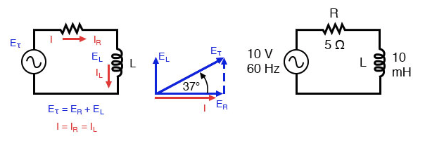
Series resistor inductor circuit: Current lags applied voltage by 0o to 90o.
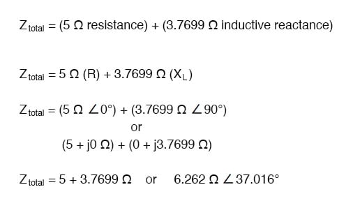
The resistor will offer 5 Ω of resistance to AC current regardless of frequency, while the inductor will offer 3.7699 Ω of reactance to AC current at 60 Hz.
Because the resistor’s resistance is a real number (5 Ω ∠ 0°, or 5 + j0 Ω), and the inductor’s reactance is an imaginary number (3.7699 Ω ∠ 90°, or 0 + j3.7699 Ω), the combined effect of the two components will be an opposition to current equal to the complex sum of the two numbers.
This combined opposition will be a vector combination of resistance and reactance. In order to express this opposition succinctly, we need a more comprehensive term for opposition to current than either resistance or reactance alone.
This term is called impedance, its symbol is Z, and it is also expressed in the unit of ohms, just like resistance and reactance. In the above example, the total circuit impedance is:
Resistance in Ohm’s Law
Impedance is related to voltage and current just as you might expect, in a manner similar to resistance in Ohm’s Law:
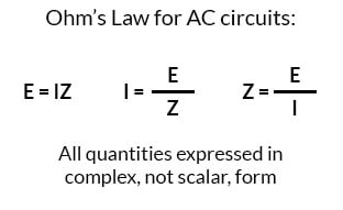
In fact, this is a far more comprehensive form of Ohm’s Law than what was taught in DC electronics (E=IR), just as impedance is a far more comprehensive expression of opposition to the flow of current than resistance is. Any resistance and any reactance, separately or in combination (series/parallel), can be and should be represented as a single impedance in an AC circuit.
To calculate current in the above circuit, we first need to give a phase angle reference for the voltage source, which is generally assumed to be zero. (The phase angles of resistive and inductive impedance are always 0° and +90°, respectively, regardless of the given phase angles for voltage or current).
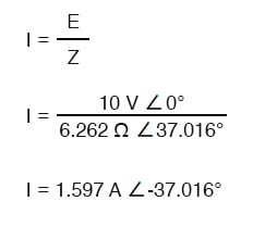
As with the purely inductive circuit, the current wave lags behind the voltage wave (of the source), although this time the lag is not as great: only 37.016° as opposed to a full 90° as was the case in the purely inductive circuit.
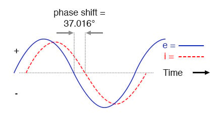
Current lags voltage in a series L-R circuit.
For the resistor and the inductor, the phase relationships between voltage and current haven’t changed. The voltage across the resistor is in phase (0° shift) with the current through it, and the voltage across the inductor is +90° out of phase with the current going through it. We can verify this mathematically:
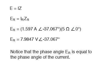
The voltage across the resistor has the exact same phase angle as the current through it, telling us that E and I are in phase (for the resistor only).
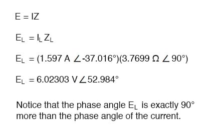
The voltage across the inductor has a phase angle of 52.984°, while the current through the inductor has a phase angle of -37.016°, a difference of exactly 90° between the two. This tells us that E and I are still 90° out of phase (for the inductor only).
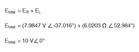
Use the Kirchhoff’s Voltage Law
We can also mathematically prove that these complex values add together to make the total voltage, just as Kirchhoff’s Voltage Law would predict:
6.4 Parallel Resistor-Inductor Circuits
Let’s take the same components for our series example circuit and connect them in parallel:
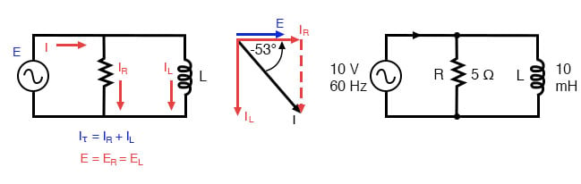
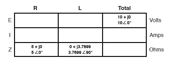
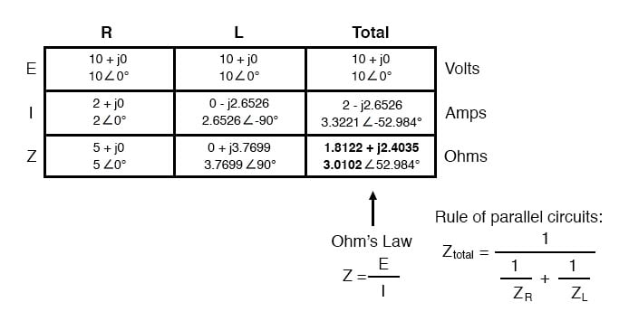
Because the power source has the same frequency as the series example circuit, and the resistor and inductor both have the same values of resistance and inductance, respectively, they must also have the same values of impedance. So, we can begin our analysis table with the same “given” values:
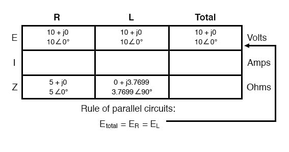
The only difference in our analysis technique this time is that we will apply the rules of parallel circuits instead of the rules for series circuits. The approach is fundamentally the same as for DC. We know that voltage is shared uniformly by all components in a parallel circuit, so we can transfer the figure of total voltage (10 volts ∠ 0°) to all component columns:
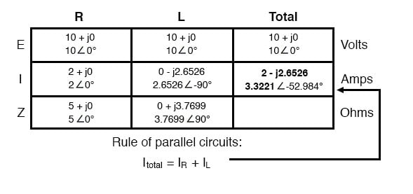
Now we can apply Ohm’s Law (I=E/Z) vertically to two columns of the table, calculating current through the resistor and current through the inductor:

Just as with DC circuits, branch currents in a parallel AC circuit add to form the total current (Kirchhoff’s Current Law still holds true for AC as it did for DC):
Finally, total impedance can be calculated by using Ohm’s Law (Z=E/I) vertically in the “Total” column. Incidentally, parallel impedance can also be calculated by using a reciprocal formula identical to that used in calculating parallel resistances.
The only problem with using this formula is that it typically involves a lot of calculator keystrokes to carry out. And if you’re determined to run through a formula like this “longhand,” be prepared for a very large amount of work! But, just as with DC circuits, we often have multiple options in calculating the quantities in our analysis tables, and this example is no different. No matter which way you calculate total impedance (Ohm’s Law or the reciprocal formula), you will arrive at the same figure:
- Impedances (Z) are managed just like resistances (R) in parallel circuit analysis: parallel impedances diminish to form the total impedance, using the reciprocal formula. Just be sure to perform all calculations in complex (not scalar) form!
[latex]Z_{parallel}=\frac{1}{(\frac{1}{Z1} + \frac{1}{Z2} + . . . \frac{1}{Zn})}[/latex]
- Ohm’s Law for AC circuits:
[latex]E = {I}{Z}[/latex] ; [latex]I = \frac{E}{Z}[/latex] ; [latex]Z =\frac{E}{I}[/latex]
- When resistors and inductors are mixed together in parallel circuits (just as in series circuits), the total impedance will have a phase angle somewhere between 0° and +90°. The circuit current will have a phase angle somewhere between 0° and -90°.
- Parallel AC circuits exhibit the same fundamental properties as parallel DC circuits: voltage is uniform throughout the circuit, branch currents add to form the total current, and impedances diminish (through the reciprocal formula) to form the total impedance.
6.5 Inductor Quirks
In an ideal case, an inductor acts as a purely reactive device. That is, its opposition to AC current is strictly based on inductive reaction to changes in current, and not electron friction as is the case with resistive components. However, inductors are not quite so pure in their reactive behavior. To begin with, they’re made of wire, and we know that all wire possesses some measurable amount of resistance (unless its superconducting wire). This built-in resistance acts as though it were connected in series with the perfect inductance of the coil, like this:
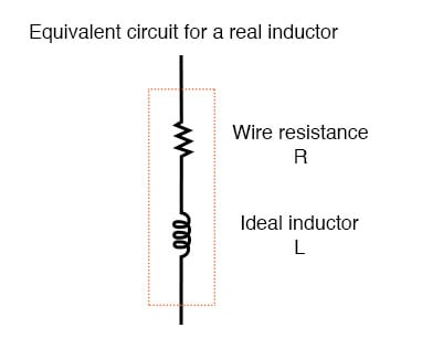
Figure 6.8 Inductor Equivalent circuit of a real inductor.
Consequently, the impedance of any real inductor will always be a complex combination of resistance and inductive reactance.
Compounding this problem is something called the skin effect, which is AC’s tendency to flow through the outer areas of a conductor’s cross-section rather than through the middle. When electrons flow in a single direction (DC), they use the entire cross-sectional area of the conductor to move. Electrons switching directions of flow, on the other hand, tend to avoid travel through the very middle of a conductor, limiting the effective cross-sectional area available. The skin effect becomes more pronounced as frequency increases.
Also, the alternating magnetic field of an inductor energized with AC may radiate off into space as part of an electromagnetic wave, especially if the AC is of high frequency. This radiated energy does not return to the inductor, and so it manifests itself as resistance (power dissipation) in the circuit.
Added to the resistive losses of wire and radiation, there are other effects at work in iron-core inductors which manifest themselves as additional resistance between the leads. When an inductor is energized with AC, the alternating magnetic fields produced tend to induce circulating currents within the iron core known as eddy currents. These electric currents in the iron core have to overcome the electrical resistance offered by the iron, which is not as good a conductor as copper. Eddy current losses are primarily counteracted by dividing the iron core up into many thin sheets (laminations), each one separated from the other by a thin layer of electrically insulating varnish. With the cross-section of the core divided up into many electrically isolated sections, current cannot circulate within that cross-sectional area and there will be no (or very little) resistive losses from that effect.
As you might have expected, eddy current losses in metallic inductor cores manifest themselves in the form of heat. The effect is more pronounced at higher frequencies, and can be so extreme that it is sometimes exploited in manufacturing processes to heat metal objects! In fact, this process of “inductive heating” is often used in high-purity metal foundry operations, where metallic elements and alloys must be heated in a vacuum environment to avoid contamination by air, and thus where standard combustion heating technology would be useless. It is a “non-contact” technology, the heated substance not having to touch the coil(s) producing the magnetic field.
In high-frequency service, eddy currents can even develop within the cross-section of the wire itself, contributing to additional resistive effects. To counteract this tendency, special wire made of very fine, individually insulated strands called Litz wire (short for Litzendraht) can be used. The insulation separating strands from each other prevent eddy currents from circulating through the whole wire’s cross-sectional area.
Additionally, any magnetic hysteresis that needs to be overcome with every reversal of the inductor’s magnetic field constitutes an expenditure of energy that manifests itself as resistance in the circuit. Some core materials (such as ferrite) are particularly notorious for their hysteretic effect. Counteracting this effect is best done by means of proper core material selection and limits on the peak magnetic field intensity generated with each cycle.
Altogether, the stray resistive properties of a real inductor (wire resistance, radiation losses, eddy currents, and hysteresis losses) are expressed under the single term of “effective resistance:”
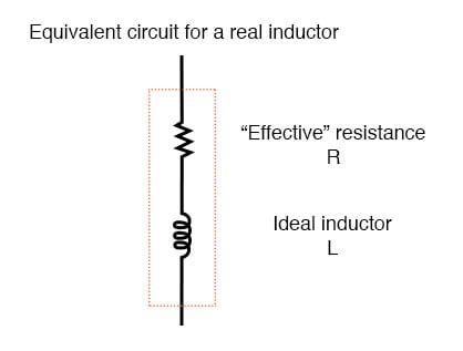
Figure 6.9 Equivalent circuit of a real inductor with skin-effect, radiation, eddy current, and hysteresis losses.
It is worthy to note that the skin effect and radiation losses apply just as well to straight lengths of wire in an AC circuit as they do a coiled wire. Usually, their combined effect is too small to notice, but at radio frequencies, they can be quite large. A radio transmitter antenna, for example, is designed with the express purpose of dissipating the greatest amount of energy in the form of electromagnetic radiation.
6.6 AC Capacitor Circuits
Capacitors Vs. Resistors
Capacitors do not behave the same as resistors. Whereas resistors allow a flow of electrons through them directly proportional to the voltage drop, capacitors oppose changes in voltage by drawing or supplying current as they charge or discharge to the new voltage level. The flow of electrons “through” a capacitor is directly proportional to the rate of change of voltage across the capacitor. This opposition to voltage change is another form of reactance, but one that is precisely opposite to the kind exhibited by inductors.
Capacitor Circuit Characteristics
Expressed mathematically, the relationship between the current “through” the capacitor and rate of voltage change across the capacitor is as such:
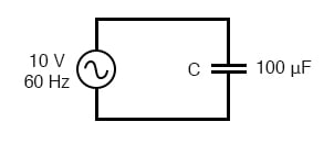
The expression de/dt is one from calculus, meaning the rate of change of instantaneous voltage (e) over time, in volts per second. The capacitance (C) is in Farads, and the instantaneous current (i), of course, is in amps. Sometimes you will find the rate of instantaneous voltage change over time expressed as dv/dt instead of de/dt: using the lower-case letter “v” instead or “e” to represent voltage, but it means the exact same thing. To show what happens with alternating current, let’s analyze a simple capacitor circuit:
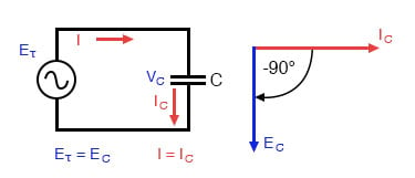
Figure 6.10 Pure capacitive circuit: capacitor voltage lags capacitor current by 90°
If we were to plot the current and voltage for this very simple circuit, it would look something like this:
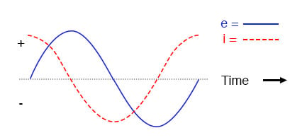
Figure 6.11 Pure capacitive circuit waveforms.
Remember, the current through a capacitor is a reaction against the change in voltage across it. Therefore, the instantaneous current is zero whenever the instantaneous voltage is at a peak (zero change, or level slope, on the voltage sine wave), and the instantaneous current is at a peak wherever the instantaneous voltage is at maximum change (the points of steepest slope on the voltage wave, where it crosses the zero line). This results in a voltage wave that is -90° out of phase with the current wave. Looking at the graph, the current wave seems to have a “head start” on the voltage wave; the current “leads” the voltage, and the voltage “lags” behind the current.
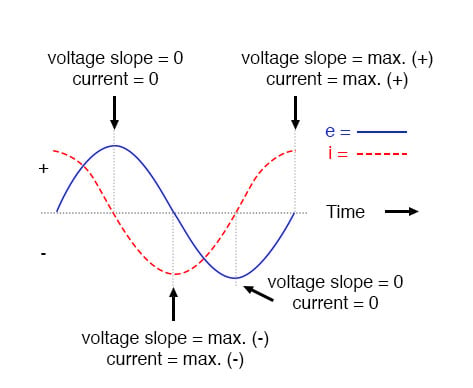
Figure 6.12 Voltage lags current by 90° in a pure capacitive circuit.
As you might have guessed, the same unusual power wave that we saw with the simple inductor circuit is present in the simple capacitor circuit, too:
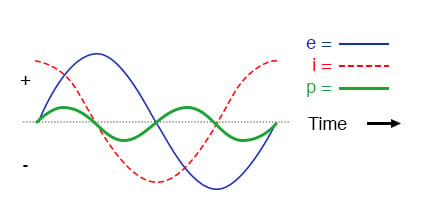
Figure 6.13 In a pure capacitive circuit, the instantaneous power may be positive or negative.
As with the simple inductor circuit, the 90-degree phase shift between voltage and current results in a power wave that alternates equally between positive and negative. This means that a capacitor does not dissipate power as it reacts against changes in voltage; it merely absorbs and releases power, alternately.
A Capacitor’s Reactance
A capacitor’s opposition to change in voltage translates to an opposition to alternating voltage in general, which is by definition always changing in instantaneous magnitude and direction. For any given magnitude of AC voltage at a given frequency, a capacitor of given size will “conduct” a certain magnitude of AC current. Just as the current through a resistor is a function of the voltage across the resistor and the resistance offered by the resistor, the AC current through a capacitor is a function of the AC voltage across it, and the reactance offered by the capacitor. As with inductors, the reactance of a capacitor is expressed in ohms and symbolized by the letter X (or XC to be more specific).
Since capacitors “conduct” current in proportion to the rate of voltage change, they will pass more current for faster-changing voltages (as they charge and discharge to the same voltage peaks in less time), and less current for slower-changing voltages. What this means is that reactance in ohms for any capacitor is inversely proportional to the frequency of the alternating current.
Reactance of a 100 uF capacitor:
| Frequency (Hertz) | Reactance (Ohms) |
| 60 | 26.5258 |
| 120 | 13.2629 |
| 2500 | 0.6366 |
Please note that the relationship of capacitive reactance to frequency is exactly opposite from that of inductive reactance. Capacitive reactance (in ohms) decreases with increasing AC frequency. Conversely, inductive reactance (in ohms) increases with increasing AC frequency. Inductors oppose faster changing currents by producing greater voltage drops; capacitors oppose faster changing voltage drops by allowing greater currents.
As with inductors, the reactance equation’s 2πf term may be replaced by the lowercase Greek letter Omega (ω), which is referred to as the angular velocity of the AC circuit. Thus, the equation XC = 1/(2πfC) could also be written as XC = 1/(ωC), with ω cast in units of radians per second.
Alternating current in a simple capacitive circuit is equal to the voltage (in volts) divided by the capacitive reactance (in ohms), just as either alternating or direct current in a simple resistive circuit is equal to the voltage (in volts) divided by the resistance (in ohms). The following circuit illustrates this mathematical relationship by example:
Examples 6.3
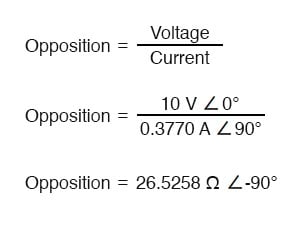
Capacitive reactance.
[latex]X_C = 26.5258Ω[/latex]
[latex]I=\frac{E}{X}[/latex]
[latex]I=\frac{10}{26.5258Ω}[/latex]
[latex]I=0.3770A[/latex]
However, we need to keep in mind that voltage and current are not in phase here. As was shown earlier, the current has a phase shift of +90° with respect to the voltage. If we represent these phase angles of voltage and current mathematically, we can calculate the phase angle of the capacitor’s reactive opposition to current.
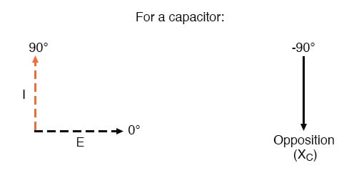
Voltage lags current by 90° in a capacitor.
Mathematically, we say that the phase angle of a capacitor’s opposition to current is -90°, meaning that a capacitor’s opposition to current is a negative imaginary quantity. (See figure above.) This phase angle of reactive opposition to current becomes critically important in circuit analysis, especially for complex AC circuits where reactance and resistance interact. It will prove beneficial to represent any component’s opposition to current in terms of complex numbers, and not just scalar quantities of resistance and reactance.
Review
- Capacitive reactance is the opposition that a capacitor offers to alternating current due to its phase-shifted storage and release of energy in its electric field. Reactance is symbolized by the capital letter “X” and is measured in ohms just like resistance (R).
- Capacitive reactance can be calculated using this formula: XC = 1/(2πfC)
- Capacitive reactance decreases with increasing frequency. In other words, the higher the frequency, the less it opposes (the more it “conducts”) AC current.
6.7 Parallel Resistor-Capacitor Circuits
Using the same value components in our series example circuit, we will connect them in parallel and see what happens:
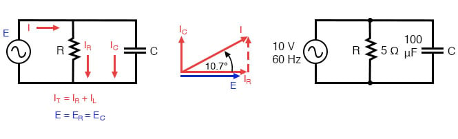
Figure 6.14 Parallel R-C circuit.
Resistor and Capacitor in Parallel
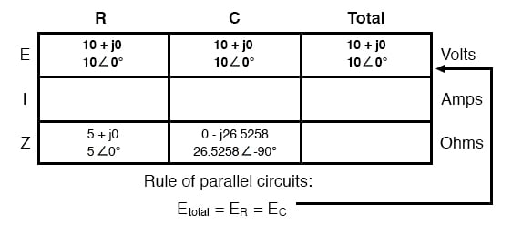
Because the power source has the same frequency as the series example circuit, and the resistor and capacitor both have the same values of resistance and capacitance, respectively, they must also have the same values of impedance. So, we can begin our analysis table with the same “given” values:
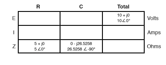
This being a parallel circuit now, we know that voltage is shared equally by all components, so we can place the figure for total voltage (10 volts ∠ 0°) in all the columns:
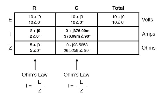
Calculation Using Ohm’s Law
Now we can apply Ohm’s Law (I=E/Z) vertically to two columns in the table, calculating current through the resistor and current through the capacitor:
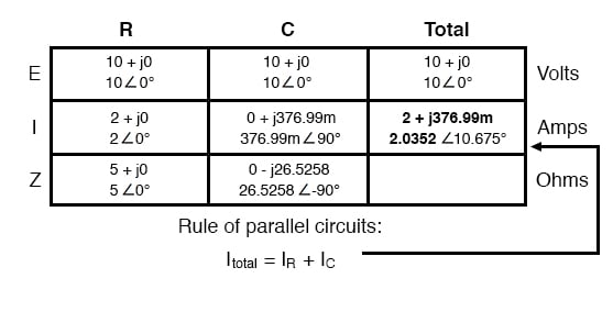
Just as with DC circuits, branch currents in a parallel AC circuit add up to form the total current (Kirchhoff’s Current Law again):
Finally, total impedance can be calculated by using Ohm’s Law (Z=E/I) vertically in the “Total” column. As we saw in the AC inductance chapter, parallel impedance can also be calculated by using a reciprocal formula identical to that used in calculating parallel resistances. It is noteworthy to mention that this parallel impedance rule holds true regardless of the kind of impedances placed in parallel. In other words, it doesn’t matter if we’re calculating a circuit composed of parallel resistors, parallel inductors, parallel capacitors, or some combination thereof: in the form of impedances (Z), all the terms are common and can be applied uniformly to the same formula. Once again, the parallel impedance formula looks like this:
The only drawback to using this equation is the significant amount of work required to work it out, especially without the assistance of a calculator capable of manipulating complex quantities. Regardless of how we calculate total impedance for our parallel circuit (either Ohm’s Law or the reciprocal formula), we will arrive at the same figure:
- Impedances (Z) are managed just like resistances (R) in parallel circuit analysis: parallel impedances diminish to form the total impedance, using the reciprocal formula. Just be sure to
Review
- perform all calculations in complex (not scalar) form! ZTotal = 1/(1/Z1 + 1/Z2 + . . . 1/Zn)
- Ohm’s Law for AC circuits: E = IZ ; I = E/Z ; Z = E/I
- When resistors and capacitors are mixed together in parallel circuits (just as in series circuits), the total impedance will have a phase angle somewhere between 0° and -90°. The circuit current will have a phase angle somewhere between 0° and +90°.
- Parallel AC circuits exhibit the same fundamental properties as parallel DC circuits: voltage is uniform throughout the circuit, branch currents add to form the total current, and impedances diminish (through the reciprocal formula) to form the total impedance.
6.8 Review of R, X, and Z
(The following section was adapted from: Lessons in Electric Circuits, Vol II, Chapter 5 – Reactance And Impedance — R, L, And C)
Before we begin to explore the effects of resistors, inductors, and capacitors connected together in the same AC circuits, let’s briefly review some basic terms and facts.
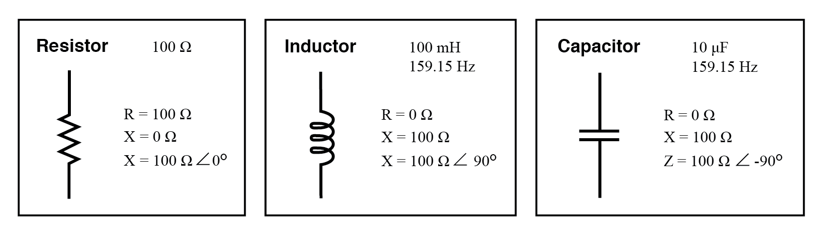
Resistance
This is essentially friction against the flow of current. It is present in all conductors to some extent (except superconductors!), most notably in resistors. When the alternating current goes through a resistance, a voltage drop is produced that is in-phase with the current. Resistance is mathematically symbolized by the letter “R” and is measured in the unit of ohms (Ω).
Reactance
This is essentially inertia against the flow of current. It is present anywhere electric or magnetic fields are developed in proportion to an applied voltage or current, respectively; but most notably in capacitors and inductors. When the alternating current goes through a pure reactance, a voltage drop is produced that is 90° out of phase with the current. Reactance is mathematically symbolized by the letter “X” and is measured in the unit of ohms (Ω).
Impedance
This is a comprehensive expression of any and all forms of opposition to current flow, including both resistance and reactance. It is present in all circuits, and in all components. When the alternating current goes through an impedance, a voltage drop is produced that is somewhere between 0° and 90° out of phase with the current. Impedance is mathematically symbolized by the letter “Z” and is measured in the unit of ohms (Ω), in complex form.
Perfect resistors possess resistance, but not reactance. Perfect inductors and perfect capacitors possess reactance but no resistance. All components possess impedance, and because of this universal quality, it makes sense to translate all component values (resistance, inductance, capacitance) into common terms of impedance as the first step in analyzing an AC circuit.
The impedance phase angle for any component is the phase shift between the voltage across that component and current through that component. For a perfect resistor, the voltage drop and current are always in phase with each other, and so the impedance angle of a resistor is said to be 0°. For a perfect inductor, voltage drop always leads current by 90°, and so an inductor’s impedance phase angle is said to be +90°. For a perfect capacitor, voltage drop always lags current by 90°, and so a capacitor’s impedance phase angle is said to be -90°.
Impedances in AC behave analogously to resistances in DC circuits: they add in series, and they diminish in parallel. A revised version of Ohm’s Law, based on impedance rather than resistance, looks like this:
Ohm’s Law for AC Circuit
[latex]\begin{align} \tag{6.2} \text{E }&={I}{Z} \\ \text{I } &=\frac{E}{Z}\\ \text{Z }&=\frac{E}{I} \end{align}[/latex]
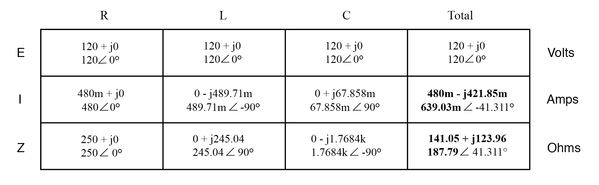
6.9 Parallel R, L, and C
We can take the same components from the series circuit and rearrange them into a parallel configuration for an easy example circuit:
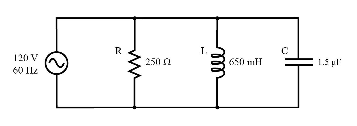
Impedance in Parallel Components
The fact that these components are connected in parallel instead of series now has absolutely no effect on their individual impedances. So long as the power supply is the same frequency as before, the inductive and capacitive reactances will not have changed at all.
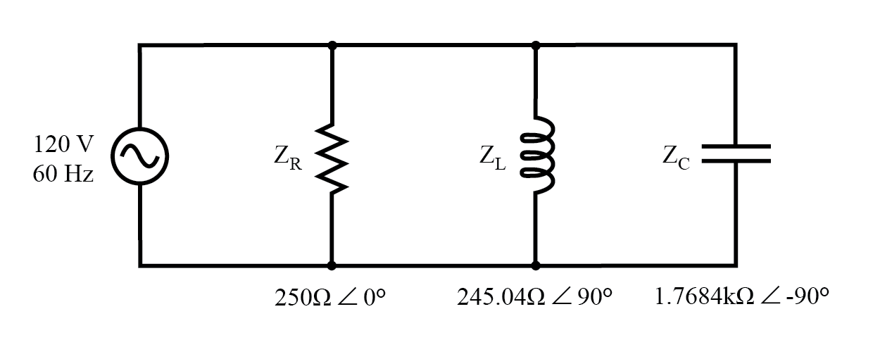
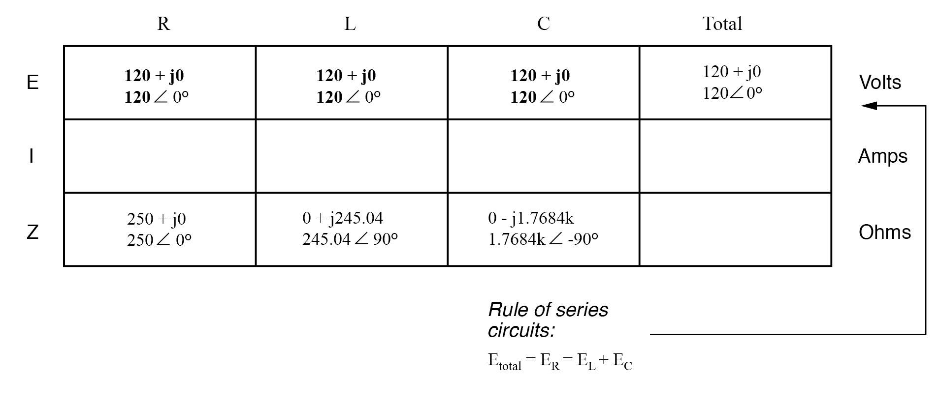
With all component values expressed as impedances (Z), we can set up an analysis table and proceed as in the last example problem, except this time following the rules of parallel circuits instead of series.
Knowing that voltage is shared equally by all components in a parallel circuit, we can transfer the figure for total voltage to all component columns in the table:
Now, we can apply Ohm’s Law (I=E/Z) vertically in each column to determine the current through each component:
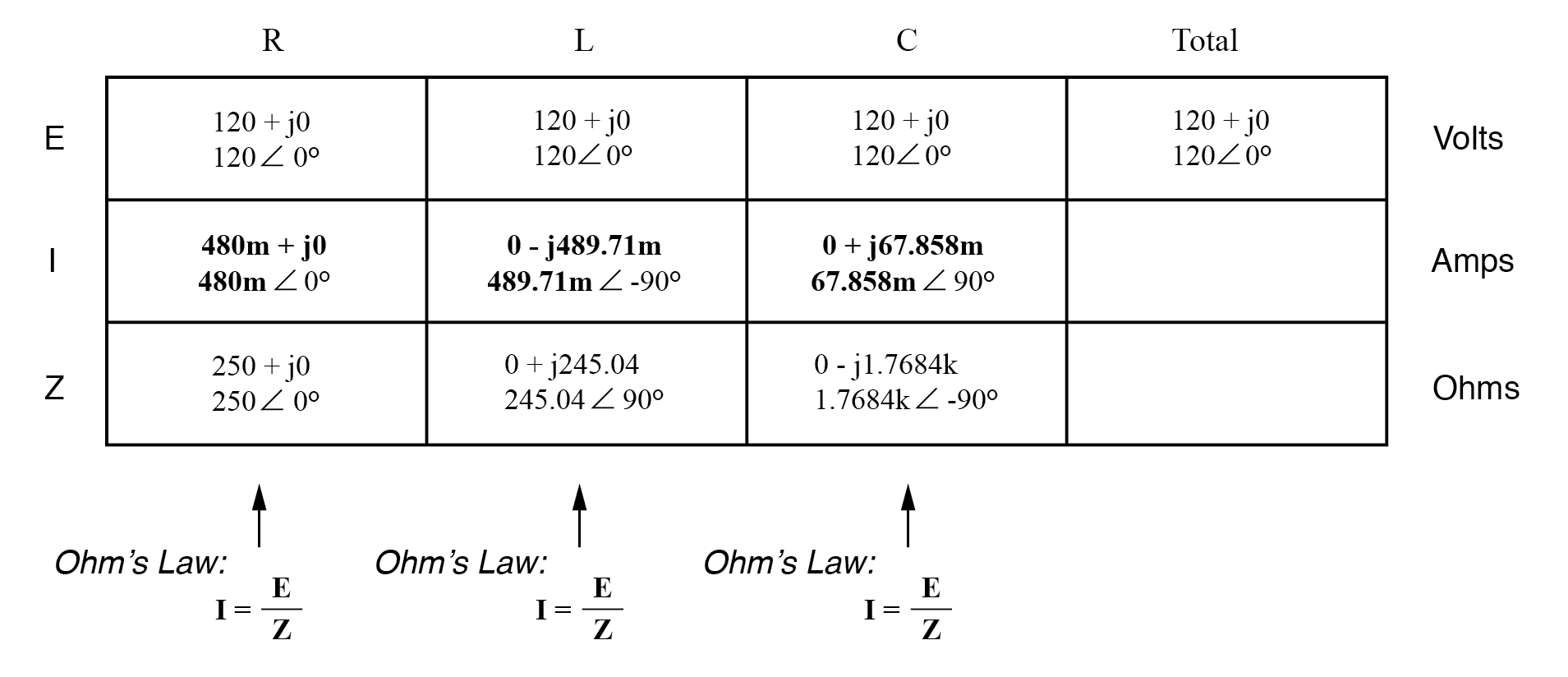
Calculation of Total Current and Total Impedance
There are two strategies for calculating the total current and total impedance. First, we could calculate total impedance from all the individual impedances in parallel (ZTotal = 1/(1/ZR + 1/ZL + 1/ZC), and then calculate total current by dividing source voltage by total impedance (I=E/Z).
However, working through the parallel impedance equation with complex numbers is no easy task, with all the reciprocations (1/Z). This is especially true if you’re unfortunate enough not to have a calculator that handles complex numbers and are forced to do it all by hand (reciprocate the individual impedances in polar form, then convert them all to rectangular form for addition, then convert back to polar form for the final inversion, then invert). The second way to calculate total current and total impedance is to add up all the branch currents to arrive at total current (total current in a parallel circuit—AC or DC—is equal to the sum of the branch currents), then use Ohm’s Law to determine total impedance from total voltage and total current (Z=E/I).
Either method, performed properly, will provide the correct answers.
6.10 R, L and C Summary
With the notable exception of calculations for power (P), all AC circuit calculations are based on the same general principles as calculations for DC circuits. The only significant difference is that fact that AC calculations use complex quantities while DC calculations use scalar quantities. Ohm’s Law, Kirchhoff’s Laws, and even the network theorems learned in DC still hold true for AC when voltage, current, and impedance are all expressed with complex numbers. The same troubleshooting strategies applied toward DC circuits also hold for AC, although AC can certainly be more difficult to work with due to phase angles which aren’t registered by a handheld multimeter.
Power is another subject altogether and will be covered in its own chapter in this book. Because the power in a reactive circuit is both absorbed and released—not just dissipated as it is with resistors—its mathematical handling requires a more direct application of trigonometry to solve.
When faced with analyzing an AC circuit, the first step in the analysis is to convert all resistor, inductor, and capacitor component values into impedances (Z), based on the frequency of the power source. After, proceed with the same steps and strategies learned for analyzing DC circuits, using the new form of Ohm’s Law: E=IZ; I=E/Z; and Z=E/I
Remember that only the calculated figures expressed in polar form apply directly to empirical measurements of voltage and current. A rectangular notation is merely a useful tool for us to add and subtract complex quantities together. Polar notation, where the magnitude (length of the vector) directly relates to the magnitude of the voltage or current measured, and the angle directly relates to the phase shift in degrees, is the most practical way to express complex quantities for circuit analysis.