Creating a map

Thinking about the logistics of making a soil map, we must come to terms with how we map something that by definition exists mostly underground. Making an accurate road map is relatively easy since the advent of aerial photography. All one has to do is trace the roads that one sees in that image and then label them. Unlike road maps, soil maps are a game of spatial prediction. A soil mapper could poke hundreds of holes in the ground and still only directly observe a small portion of the soil landscape. Aerial photographs have played a key role in the creation of soil survey maps, but they don’t let the soil mapper see much of the soil.

Traditional soil maps were created using the soil surveyor’s knowledge, intuition, and understanding of the available soil information It is impossible for farmers to sample all locations within their fields because it is unpractical and time and cost expensive. To address this problem, maps are created by making predictions at unsampled locations based on scatter observations across the landscape. Soil sampling provides a broad understanding of the soil for that specific point. However, this knowledge is useful to identify patterns and relationships among soil properties.

Spatial predictions

Our best clues for predicting soil properties come from the environment that they formed in. Recall the factors of soil formation that describe environmental variables that influence soil processes. Such factors were probably credited to Hans Jenny, but they were listed sixty years before that by Vasily Dokuchaev when he was describing how to map soil in Russia. Nobody had thought to use combinations of factors to predict soil variation. The environment, including topography, climate, and vegetation, may explain more about soil properties than we can think of. The ancient Greeks knew to look at the vegetation for clues and the German agrogeologists of the 20th century knew to look at texture and mineralogy for clues, but previously these were considered to be competing ideas.

Spatial association

Utilizing the factors of soil information to associate patterns of soil variation is known as the soil-landscape paradigm. This is a specific example of the geographic concept of spatial association, which is that some variables covary with each other in space. By looking at variables that are more readily observed, one can infer variables that aren’t as easily observed. In the case of the soil landscape paradigm, a soil mapper could observe soil properties in one location and infer that other locations with matching climate, vegetation (the part of organisms that can be seen in an aerial photograph), landscape position, and parent material would also have the same combination of soil properties. For example, the Clarion soil series is mapped on the tops of the gentle hills of the Dows geologic formation (region known as the Des Moines Lobe). Within a county scale map, climate doesn’t change very much. However, there are measurable differences in climate across multiple counties. For this reason, the Clarion soil series is not associated with exactly the same soil properties from one county to the next. Although parallel in the other factors of soil formation, the Clarion soil series is associated with slightly different soil properties as observed in each county and the same is done for all soil series. This strategy allows for a general concept of soil series to be easily communicated, while also helping the county soil maps to be more accurate.

Spatial association with a machine learning approach

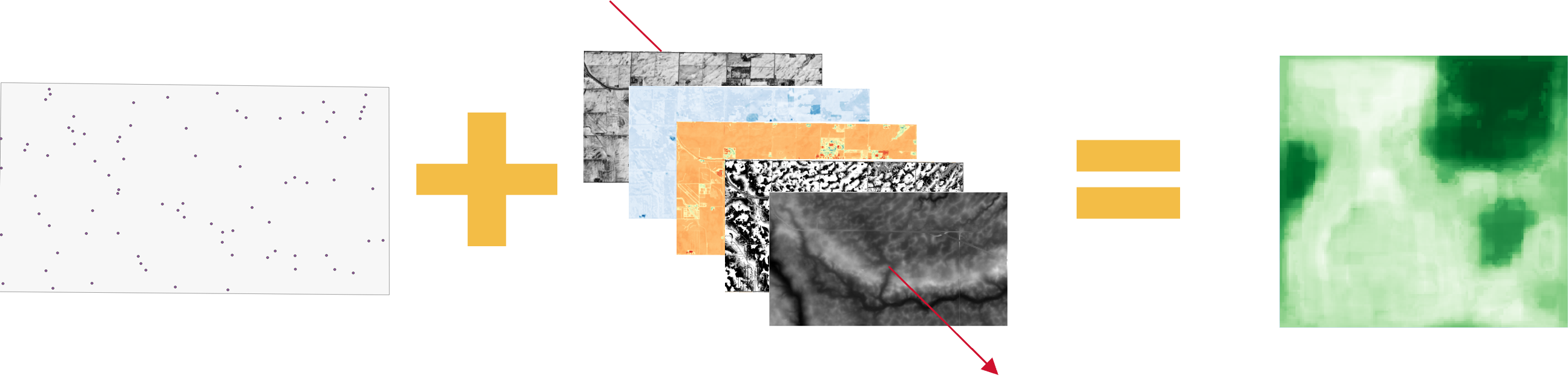
Artificial intelligence is a power and modern tool that has supported and improved the creation of high-quality maps. The idea behind this method is make spatial predictions at unsampled locations by recognizing relationships between known values and some ancillary data (covariates). Such covariates include topography, vegetation, satellite imagery or even other soil maps that may provide enough background information to explain soil’s behavior at the locations where predictions want to be made. Different machine learning algorithms arrange the data at a specific known location and associate it with the covariates for that same point. The machine learning algorithm fits a model over that data and help make predictions of unknown values at unsampled locations. The following image represents the process:

 

Spatial autocorrelation

To make soil fertility maps, all the same basic principles apply for mapping something that we can only directly observe in a few locations while wanting to know the spatial distribution of that target variable across the whole map area. We still must predict the status of the soil belowground based on a small proportion of samples and whatever clues we can find aboveground. Because dynamic soil properties are changing quickly and with them their relationships to aboveground variables, soil fertility mapping tends to lean on a different geographic principle. This other principle is spatial autocorrelation, which means that things that are close together tend to be more similar to each other than things that are farther away. By this principle, two measurements of soil nitrate concentrations taken 3 feet (1 meter) apart are more likely to be similar that two samples taken 100 feet (30 meters) apart. Now, any soil scientist will tell you that you can be surprised by differences in soil cores taken almost side by side, and in the case of soil fertility you want to be careful not to sample on a hot spot where fertilizer was recently applied (e.g., the thin band produced by targeted side-dressing). However, part of being a dynamic soil property is being relatively more mobile than static soil properties and that lends to more diffuse spatial distributions. Not having hard breaks in concentrations works better for the spatial autocorrelation approach to mapping.

The most basic method for using spatial autocorrelation to create a map is to take the sample points and then draw polygons identifying the area closest to the respective points. This identifies the areas that are likely to be similar to each of those measured points. Then we assign the measured value of each point to its respective surrounding area. In doing this, we are predicting values in an area based on the nearest measured location. A common practice in soil fertility mapping is to take soil samples on a regular grid, and then assign sample results to equally size squares surrounding each of the sample points. Although variability likely exists within those squares, if the squares are not larger than the size of area that a farmer can vary their management practices, then a finer resolution would not be useful.

In the era of precision agriculture, rates of applying soil amendments can be increasingly targeted. This means that a 2.5-acre grid (100 x 100 m squares) or even a 1-acre grid (60 x 60 m squares) may be too coarse of a resolution to supply the information needed to fully utilize the capabilities of precision agriculture. With the basic spatial autocorrelation approach described above, making a finer resolution map would require taking more soil samples. Instead of a sample in every acre, maybe management zones of 0.5 acre can have unique fertilizer prescriptions. In which case, a sample in every 0.5 acre would double the quantity of samples needed. However, spatial autocorrelation can be more useful than single value blocks. Spatial interpolation uses the concept of spatial autocorrelation to predict a smoother gradient of values in between observed locations. Within a geographic computer-based software, algorithms such as inverse distance weighting (IDW) or kriging can create prediction surfaces at any resolution the user specifies.

Spatial autocorrelation approach (variogram)

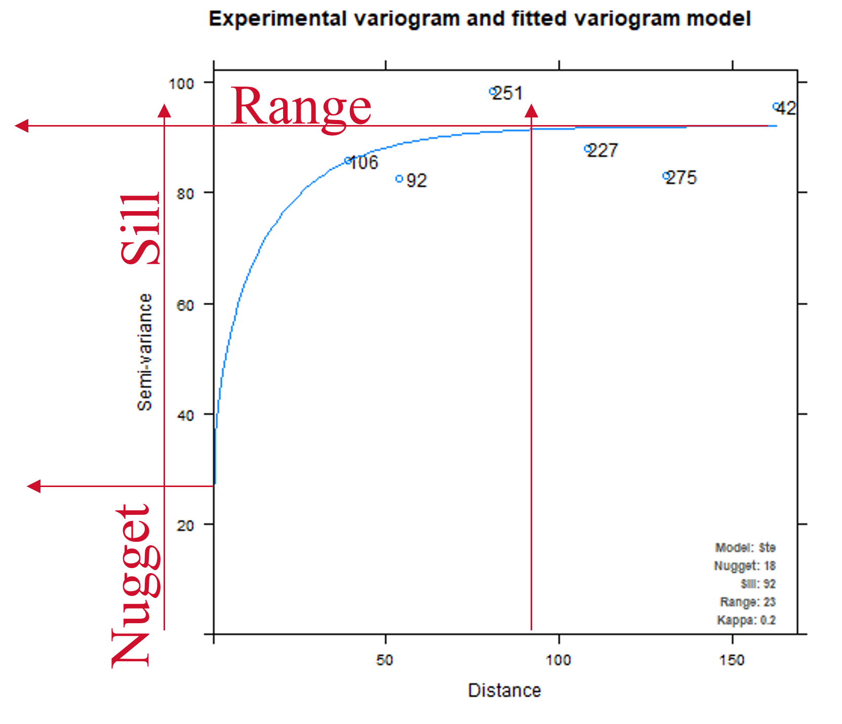
The variogram is the statistical tool used with kriging methods to predict values at unsampled locations based on distance from a known point. It tells how much two samples can vary based on the distance that exists between them. The range is the distance at which the variogram levels off and points at this distance or farther apart are not spatially correlated. The nugget effect is a representation of the small-scale variability, and the sill is the maximum variability between a pair of points. In this example, a model was fitted into a variogram while performing an ordinary kriging analysis for Phosphorus content in the soil. The model fitted into the variogram is telling us how much the data is expected to vary as the distance from a point starts increasing (lag distance in x axis).

 

Geographic Information Systems (GIS)

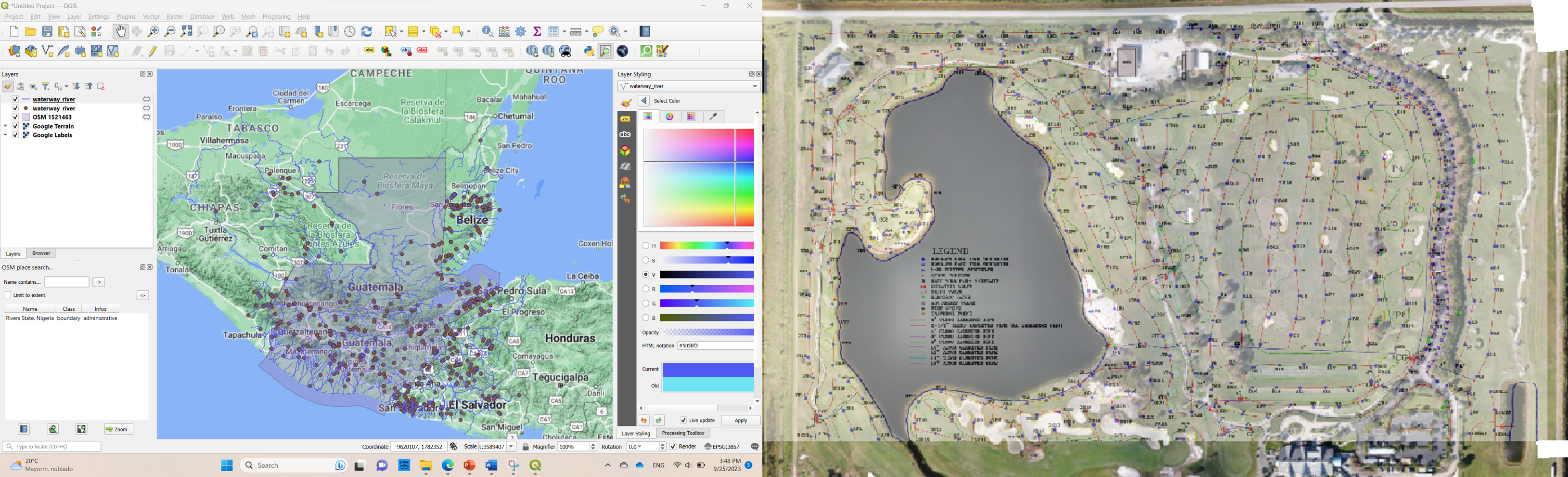
The acronym GIS stands for Geographical Information Systems. GIS is the implementation of software and hardware for the storage and manipulation of spatial data. Digital geographers combine computing power and computer-based analysis to store, modify, analyze, and present geographic data using digital maps. Its capabilities allow users to even tie non-spatial data to a specific location and obtain geographical results. For example, a list of coffee shops does not provide much information beyond the name of each and probably an idea of what they sell. However, if a set of coordinates is assigned to each of those names, it is possible to locate them in space and navigate towards each.

To store and manipulate data, GIS utilizes layers of information to simplify the process. Each one of these layers includes objects with georeferenced data (data assigned to a fixed location), and values (quantitative or qualitative). Objects include:

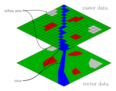
• – Vector data, or discrete objects. Each one of the items in each vector layer contains a fixed value for a certain location, it assumes the feature remains constant throughout space. Vector data can be represented by points (simple set of coordinates), lines (continuum of points), or polygons (objects that form a closed area defined by connecting lines). Commonly these are used to represent soil sample locations, stores, cities, roads, streams, or regional boundaries.
• – Raster data, or continuous objects. Because object values can vary over space (e.g., soil properties), independent locations are included at all locations of the study area. A raster is an image created by a composition of grid-arranged squared cells. Each one of the cells is called a pixel, has a unique absolute location, an individual value, and the same size as all other cells. More pixel density per area increases the level of detail, resulting in smoother images. When pixel size increases, the resolution of the map reduces and gives it a blockier appearance.

The process of obtaining data is either done by directly evaluating the object by touching it or evaluating it from a certain distance. Direct measurements of certain feature are obtained with in-field sensors. In agriculture such measurements can be either from the soil (e.g., moisture readings) or the crop (e.g., chlorophyll-meter). As an alternative, remote sensing allows farmers to obtain data from a distance. This includes images from drones, planes, or satellites, which can measure topography or spectral bands (color). Actually, both are being combined with GIS and artificial intelligence methods to increase the quality of the maps.

Raster vs. Vector data

 

Because raster pixels have a square shape, they cannot represent other geometry than that. Therefore, rasters fail to perfectly delineate non-squared objects. Instead, vector objects can delineate any figure better because the main unit is the point and by arranging infinite amounts of points, any shape can be delineated. Vector polygons may provide a better alternative for delineating irregular objects, but they assign a uniform value to the are enclosed within and detail is lost. On the contrary, because rasters can include infinite number of pixels, they are able to capture all the variability that exists within certain area. Soil survey maps that have been digitized are composed of vector objects. Each one of the lines enclosing a certain region assumes that all the area inside is homogeneous. Instead, rasters allow to capture any kind of heterogeneity that exists, especially with dynamic soil properties like nitrogen.

One of the most valuable things about GIS is that scale is no longer a problem. Instead of scale being limited by the map’s extent, in GIS it is possible to zoom in and out of the object and increase the level of detail that can be seen. This does not mean that GIS has better resolution than paper maps. Resolution is still limited by the availability of data and density of it. The difference with paper maps is that to fit a large region within a paper, the level of detail was compressed so intensely that it lost usability, especially with new Precision agriculture technologies. Now, GIS allows the user to zoom in and be able to see that detail that was lost in the transcription to paper maps. Nevertheless, if the smallest unit of sampling represents 1km2, for example, GIS won’t be able to see beyond that and all the area will be represented by a big pixel of 1 km2 of resolution.