
Plant Breeding Basics
William Beavis and Anthony Assibi Mahama
The materials in this chapter cover the basics of plant breeding and data management and analysis concepts to serve as a refresher for helping the reader prepare to work through the main chapters of the book. Some readers may find it necessary to consult some introductory breeding and statistics texts for additional preparation.
Place plant breeding activities within a framework of three categories based on goals:
- Genetic improvement
- Cultivar development
- Product placement
Defining Plant Breeding
Plant Breeding has many definitions. A working definition to consider:
Plant Breeding is the genetic improvement of crop species.
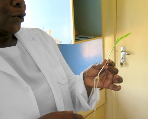
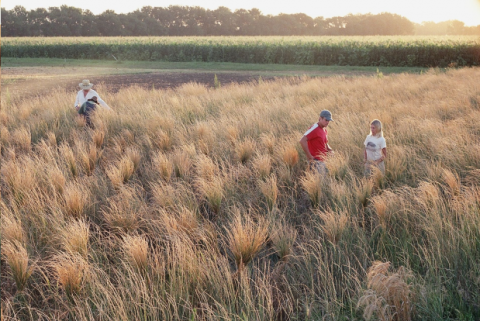
This definition implies that a process (breeding) is applied to a crop, resulting in genetic changes that are valued because they confer desirable characteristics to the crop (Fig 1). Current breeding programs are the result of thousands of years of refinements that have been implemented through considerable trial and error. Refinements to the breeding processes are constrained by limited resources, technologies, and the reproductive biology of the species. Thus, the challenge of designing a plant breeding program might be thought of as the engineering counterpart to plant science (Fig. 2).

Other definitions
- Art of plant breeding: “… the ability to discern fundamental differences of importance in the plant material available and to select and increase the more desirable types…” Hayes and Immer (1942)
- “Plant breeding, broadly defined, is the art and science of improving the genetic pattern of plants in relation to their economic use.” Smith (1966).
- “Plant breeding is the science, art, and business of improving plants for human benefit.” Bernardo (2002).
Organization of Plant Breeding Activities
For the purposes of applying appropriate quantitative genetic models in plant breeding, it is important to understand the distinctions among three types of plant breeding projects: genetic improvement, cultivar development, and product placement. The distinctions among these three types of projects are nuanced aspects of every plant breeding program, yet the distinctions are critical for applying the correct models for data analyses used in decision-making.
Cultivar Development
The primary goal of a genetic improvement (red arrows) project is to identify lines to cycle into the breeding nursery (Fig. 3) for purposes of genetic improvement of the breeding population. Identification of lines to select is accomplished through assays of segregating lines (synthetics, hybrids) with trait-based markers and small plot field trials in single and Multi-Environment field Trials (METs) (Fig. 4). Data analyses will include analyses of binary traits with binomial and multinomial models and quantitative traits with mixed linear models, where the segregating lines will be modeled as random effects and the environments as fixed effects.
The primary goal of the cultivar development project (blue filters) is to identify cultivars that have the potential to be grown throughout a targeted population of environments. Thus, in a cultivar development project, selected lines from segregating populations will be evaluated for quantitative traits in multi-environment trials. Data analyses in the Regional Trials of a cultivar development project will also be based on mixed linear models. However, in this case, lines are often modeled as fixed effects, while the environments are modeled as random effects.
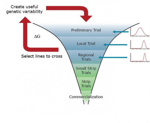
The goals of a product placement project are again distinct from genetic improvement and cultivar development. In a product placement project, agronomic management practices, as well as cultivars, are selected for the field trials. These are often organized in hierarchical (split-plot) experimental designs. Thus, the parameters of a mixed linear model associated with agronomic practices and cultivars will be modeled as fixed effects, while various levels of residual variability associated with split-plot experimental units will be modeled as random effects.
For an introductory course on Quantitative Genetics, we will focus primarily on genetic improvement, a little bit on cultivar development projects, and no time will be spent on product placement projects.
Decision-Making Process
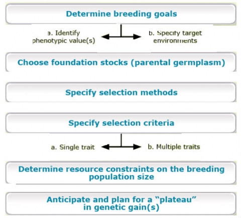
Conceptually, genetic improvement consists of a simple two-step, iterative decision-making process (Fig. 5):
1) selection of parents for crosses and 2) evaluation of their segregating progeny for the next generation of parents and development of cultivars (Fehr, 1991). Operational implementation of genetic improvements for any given species requires far more detail.
For example, Comstock (1978) outlined the major activities involved in genetic improvement by plant breeders (below).
The details of any particular breeding program will likely consist of many activities. At the same time, it is important to categorize these activities according to the goals that transcend all plant breeding programs.
A Brief History of Quantitative Genetics
Quantitative genetics addresses the challenge of connecting traits measured on quantitative scales with genes that are inherited and measured as discrete units. This challenge was originally addressed through the development of theory between 1918 and 1947. The theory is now referred to as the modern synthesis and required another 50 years for technological innovations and experimental biologists to validate. Luminaries such as RA Fisher, Sewell Wright, JBS Haldane, and John Maynard Smith were able to develop this theory without the benefit of high throughput ‘omics’ technologies. Indeed, modern synthesis was developed before knowledge of the structure of DNA.
Unlike animal breeders, plant breeders implement breeding processes in organisms that cannot be protected from highly variable environments. Because plants are rooted in the sites in which they are planted, they have evolved unique adaptive mechanisms, including whole-genome duplications that enable biochemical diversity through secondary metabolism and multiple forms of reproductive biology.
Because of the reproductive and biochemical diversity in domesticated crops, plant breeders felt little need to develop quantitative genetics beyond initial concepts associated with the Analysis of Variance (ANOVA; Fisher, 1925; 1935). Thus, plant breeders focused their efforts on the development of field plot designs and careful plot management practices to ensure balance in field plot data for ANOVA.
Modern Synthesis Theory
The lack of reproductive and biochemical diversity in animal species created constraints that forced animal breeders to concentrate their efforts on the development of quantitative genetics beyond the ideas of Fisher (1918, 1928). JL Lush (1948) and his student CR Henderson (1975) realized that genetic improvement of quantitative traits in domesticated animal species could not take advantage of replicated field trials that are based on access to cloning, inbreeding, and the ability to produce dozens to thousands of progenies per individual. With these constraints, it was not possible to obtain precise estimates of experimental error or Genotype by Environment interaction effects using classical concepts from the ANOVA. So, they developed the statistical concepts of Mixed Model Equations (MME) to estimate breeding values of individuals with statistical properties of Best Linear Unbiased Prediction (BLUP). These very powerful statistical approaches were largely ignored by plant breeders until about 1995 (Bernardo, 1996).
Marker Technologies
The power of these methods is derived from knowledge of genealogical relationships. For some commercial plant breeding organizations, genealogical information had been carefully recorded for purposes of protecting germplasm. Thus, it was relatively easy for commercial breeding companies such as Pioneer and Monsanto to implement these methods. Next, international plant breeding institutes began to incorporate mixed linear models to estimate breeding values in their genetic improvement programs (Crossa et al, 2004); again, it was fairly easy to do this with extensive pedigree information. Since about 2005, many plant quantitative geneticists have published extensively on the benefits of this approach to genetic improvement of crops (Piepho, 2009), although there remain many academic plant breeding organizations that do not utilize MME to estimate breeding values with BLUP statistical properties, primarily because pedigrees of lines developed by academic programs have not been widely shared, nor aggregated into a shared repository. In parallel to the adoption of MME by plant breeders, there has been the development of relatively inexpensive genetic marker technologies. These have enabled the use of MME for Genomic Estimates of Breeding Values (GEBV; Meuwissen, 2001), thus overcoming the lack of genealogical knowledge for many crop and tree species.
Trait Measures
Objectives: Demonstrate ability to distinguish among the various types of phenotypic and genotypic traits that are assessed routinely in a plant breeding program.
Categorical Scales
In the context of plant breeding, quantitative genetics provides us with a genetic understanding of how quantitative traits change over generations of crossing and selection. Recall traits can be evaluated on categorical (Fig. 6) or quantitative scales. If the trait of interest is evaluated based on some quality, for example, disease resistance, flower color, or developmental phase, then it is considered a categorical trait. There are three further distinctions that can be made among categorical scales:
- Binary consists of only two categories such as resistant and susceptible or small and large.
- Nominal consists of unordered categories. For example, viral disease vectors might be categorized as insects, fungi, or bacteria.
- Ordinal consists of categorical data where the order is important. For example, disease symptoms might be classified as none, low, intermediate, and severe.
Quantitative Scales
Binary, nominal, and ordinal data are typically analyzed using Generalized Linear Models. Such models require that we model the error structures using Poisson or Negative Binomial distributions and are beyond the scope of introductory quantitative genetics. It is important to remember, however, that it is not advisable to apply General Linear Models to categorical data types.
There are two further distinctions of traits that are evaluated on quantitative scales:
- Discrete data occur when there are gaps between possible values. This type of data usually involves counting. Examples include flowers per plant, number of seeds per pod, number of transcripts per sample of a developing tissue, etc.
- Continuous data can be measured and are only limited by the precision of the measuring instrument. Examples include plant height, yield per unit of land, seed weight, seed size, protein content, etc.
- In the context of measurement, Precision refers to the level of detail in the scale of the measurement.
- Accuracy refers to whether the measurement represents the true value.
Types of Models
Objectives: Be able to place plant breeding activities within a framework of three categories based on goals:
- Genetic improvement
- Cultivar development
- Product placement
Definition and Purpose of Models
Models are representations or abstractions of reality. Some models can be very useful, e.g., prediction of phenotypes, even if they are not accurate. If data are modeled well, they can be used to generate useful graphics that will inform the breeder about data quality, integrity, and novel discoveries. Most often, predictive models are in the form of mathematical functions. Also, there are models for organizing data, analyses, processes, and systems. Yes, breeding systems and genetic processes can be represented as sets of mathematical equations. Historically the subject of optimizing a breeding system has been approached through ad hoc management activities that are often tested through trial and error. In the future, design and development of plant breeding systems will need to be treated with the same rigor that engineers use to design optimal manufacturing systems. Thus, it will be important to learn how to model breeding systems as mathematical functions.
Data Modeling
Even if it were possible to record data without error, as soon as we evaluate a trait and record the value of a living organism, we lose information about the organism. The challenge is to develop a data model that will minimize recording errors and loss of information.
What Is Data Modeling?
- Data modeling is the process of defining data requirements needed to support decisions.
- Data modeling is used to assure standard, consistent, and predictable management of data as a resource for making decisions.
- Data models support data and decision systems by providing definitions and formats. If the data are modeled consistently throughout a plant breeding program, then compatibility of data can be achieved.
If a single data structure is used to store and access data, then multiple data analyses can share data.
Steps for Modeling Data in a Plant Breeding Project
- Outline the plant breeding process.
- Determine the experimental or sampling units that will be evaluated at each step in the process.
- Determine the number of experimental or sampling units that will be evaluated.
- Characterize the experimental and sampling units as well as the traits that will be evaluated at each step in the process.
An experimental unit is defined as the basic unit to which a treatment will be applied. A sampling unit is defined as a representative of a population of interest. In quantitative genetics, we evaluate responses (traits) of experimental or sampling units on continuous scales, e.g., grain yield, plant height, harvest index, etc. Note that a measurement taken on a continuous scale is not the same as a continuously measured trait. Continuously measured traits such as grain fill, transpiration, disease progression, or gene expression are measured continuously over the growth and development of an organism. Historically, evaluation of continuously changing traits has been too labor-intensive to justify their expense. The emergence of ‘phenomics’ using image processing will overcome the limitations of acquiring the data. However, the need to store and manage ‘big data’ from phenomics is going to require novel data models and computational infrastructure, or else the acquisition of such data will be meaningless.
Organizing Data
Data models address the need to organize data for subsequent analysis.
A simple data model consists of a Row x Column matrix, where all experimental or sampling units are represented in rows, and the evaluated characteristics or attributes for each unit are recorded in the columns (Fig. 7):
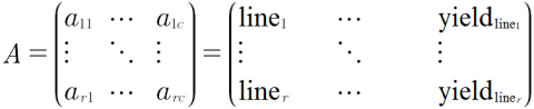
Alternatively, the Ar x c matrix can be represented as:
- A = {aij}, for i = 1,2,3 … r and j = 1,2,3 … c
- i would represent line 1, line2, line3 … line r and
- j would represent location, replication, SNP locus 1, disease rating, … yield, etc.
Preserving Data
While the A(r x c) matrix is sufficient for small research projects, it is inadequate and cumbersome for breeding programs consisting of multiple types of evaluation trials at multiple stages of development. For such programs, relational databases are designed to optimize the ability to search and prepare data for analysis and interpretation using statistic and genetic models (Fig. 7). Further unless data in an A(r x c) matrix is disseminated through “read-only” access, there is potential for alteration of originally recorded data. Thus, the use of Excel files, too commonly used to store experimental data in an A(r x c) matrix, can create serious ethical issues. While such issues do not disappear with relational databases, relational databases enable more effective protection of data as originally recorded. Recently, a publicly available database designed for organizing data from plant breeding projects has been developed. Known as the Breeding Management System, it is part of the Integrated Breeding Platform designed and developed by the Generation Challenge Program of the Consultative Group of International Agricultural Research Centers.
A Relational Database
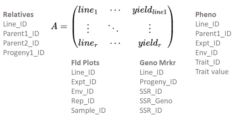
While the development of relational databases (Fig. 8) is outside of the scope of this course, it is important to note that plant breeders routinely work with database developers to design, implement, and populate relational databases.
Phenotypic Models
For the most part, plant breeders rely on linear models to represent measured traits. While we will concentrate on statistic and genetic models for continuous traits, it is important to recognize that there are well-developed data analysis methods for binary, nominal, and ordinal traits (see McCullagh and Nelder, 1989 or Christensen, 1997 for explanations of Generalized Linear Models). A general (not Generalized) linear model for the phenotype can be denoted as in Equation 1:
[latex]Y_i = \mu + e_i[/latex]
[latex]\textrm{Equation 1}[/latex] General linear model for the phenotype.
where:
[latex]Y_i[/latex] = phenotype of individual i,
[latex]\mu[/latex] = mean phenotype value of individual i,
[latex]e_i[/latex] = random variability (or lack of precision) in the measurement of the phenotype of individual i.
Further, we often assume that the variability associated with each measurement of variables, ei, is distributed as random identical and independent Normal variables. This simple model is typically associated with the hypothesis that the only source of variability is due to chance (noise). We can extend the simple model to include genetic (G) and environmental (E) sources (signals) of variability, [latex]Y = \mu + G + E +e[/latex].
Two Linear Models
Scalar Notation
We will utilize two types of models to analyze data Equations 2 and 3):
[latex]Y_i = \beta_0 + \beta_1G_1 + \epsilon_{ij}[/latex]
[latex]\textrm{Equation 2}[/latex] Linear model for phenotype.
where:
[latex]\beta_0[/latex] = intercept at the y-axis,
[latex]\beta_1[/latex] = the slope of the regression line,
[latex]G_i[/latex] = the genotypic value,
[latex]\epsilon_{ij}[/latex] = unspecified or residual sources of variability.
[latex]Y_{ij} = \mu + g_i + r_j +\epsilon_{ij}[/latex]
[latex]\textrm{Equation 3}[/latex] Linear model for phenotype.
where:
[latex]Y_{ij}[/latex] = the phenotypic response,
[latex]\mu[/latex] = the population mean,
[latex]g_i[/latex] = the genotypic unit,
[latex]r_j[/latex] = replicates of the genotypic units,
[latex]\epsilon_{ij}[/latex] = unspecified or residual sources of variability.
The parameters of Equation 2 represent the intercept and slope of a line that can be fit to data consisting of pairs of genotypic values, Gi, and phenotypic responses, where the genotypic values are continuous and known (i.e., measured without error) while the phenotypic data are measured with error in plots (experimental units). The parameters of Equation 3 represent a population mean, genotypic units, gi, rj replicates of the genotypic units, and the phenotypic, Yij responses. The genotypes are usually categorical designators of distinct segregating lines, hybrids, cultivars, clones, etc.
We typically estimate the parameters of Equations 2 and 3 using least squares methods. These methods are based on the idea of minimizing the squared differences between the model parameters and the measured phenotypic value (Equation 4). For example, using Equation 2, we want to minimize the difference as:
[latex]min(Y_i -[\beta_0 + \beta_1G_i])^2[/latex]
[latex]\textrm{Equation 4}[/latex] Model for squared differences.
where:
[latex]\textrm{terms}[/latex] are as described previously.
Taking the partial derivatives of Equation 3 with respect to β0 and β1 and setting the resulting two equations = 0, we find the slope using Equation 5:
[latex]\beta_1 = [V(G_i)]^{-1}[Cov(G_iY_i)] = \frac{[Cov(G_iY_i)]}{[V(G_i)]}\;and\ \beta_0 = \bar{Y} - \beta_1\bar{X}[/latex]
[latex]\textrm{Equation 5}[/latex] Formulae for calculating intercept and slope.
where:
[latex]V{G_i}[/latex] = the genotypic variance,
[latex]Cov{G_i Y_i}[/latex] = covariance of G and Y,
[latex]\bar{Y}[/latex] = mean of Y,
[latex]\bar{X}[/latex] = mean of X.
The result is a prediction equation (Equation 6):
[latex]\hat{Y}_i = \hat{\beta}_0 + \hat{\beta}_1X_i[/latex]</>
[latex]\textrm{Equation 6}[/latex] Prediction model.
where:
[latex]\hat{Y}, \hat{\beta_0}, \hat{\beta_1}[/latex] = the estimates of these terms,
[latex]X_i[/latex] = predictor variable, genotype, Gi.
Note that the predicted values are placed on the fitted line. Such values are sometimes referred to as ‘shrunken’ estimates because, relative to the observed values, they show much less variability.
If it were possible to obtain the true genotypic values, Gi, then we could routinely use Equation 2 to predict the phenotypic performance of individual i. Instead, plant breeders have used Equation 3 and its expanded versions to evaluate segregating lines and cultivars.
Matrix Notation
Equation 2 also can be represented by Equation 7:
[latex]y = X\beta + \epsilon\ \;\;with\ solution\ as\;\; \beta = (X'X){^{-1}}(X'\bar{Y})[/latex]
[latex]\textrm{Equation 7}[/latex] Matrix model and solution for phenotype.
where:
[latex]y[/latex] = phenotype,
[latex]X[/latex] = matrix or vector of genotype,
[latex]\epsilon[/latex] = vector or residual or error.
And Equation 3 could be represented by Equation Equation 8:
[latex]y = Xr + Zg + \upsilon[/latex]
[latex]\textrm{Equation 8}[/latex] Model for phenotype.
where:
[latex]y[/latex] = phenotype ,
[latex]X[/latex] = vector of replication,
[latex]Z[/latex] = vector of genotype.
When represented this way, though, Equation 3 is usually misinterpreted by beginning students often, as the matrix form of the equation with an added set of the parameter Z. The matrix form of Equation 2 is actually a mixed linear model equation (Equation 9) and not a simple expansion of the matrix form of Equation 1.
[latex]y = X\beta + Z\upsilon + \varepsilon[/latex]
[latex]\textrm{Equation 9}[/latex] Matrix model linear model for phenotype.
where:
[latex]y[/latex] = vector of observations (phenotypes),
[latex]X[/latex] = Incidence matrix for fixed effects,
[latex]\beta[/latex] = vector of unknown fixed effects (to be estimated),
[latex]Z[/latex] = Incidence matrix of random effects,
[latex]\upsilon[/latex] = a vector of random effects (genotypic values to be predicted),
[latex]\varepsilon[/latex] = a vector of residual errors (random effects to be predicted).
Exploratory Data Analysis (EDA)
Objectives
- Distinguish between descriptive and inferential statistics.
- Conduct and interpret exploratory data analyses.
- Distinguish parameters from estimators and estimates.
- Estimate means in both balanced and unbalanced data sets.
- Estimate variances, covariances, and correlations in balanced data sets.
Statistical Inference
The purpose of statistical inference is to interpret the data we obtain from sampling or designed experiments. Statistical Inference consists of two components: estimation and hypothesis testing. In this section, we review some introductory estimation concepts.
The purpose of statistical inference is to interpret the data we obtain from sampling or designed experiments. Preliminary insights come from graphical data summaries such as bar charts, histograms, box plots, stem-leaf plots, and simple descriptive statistics such as the range (maximum, minimum), quartiles, and the sample average, median, and mode. These exploratory data analysis (EDA) techniques should always be used prior to estimation and hypothesis testing. However, prior to conducting EDA, the phenotype should be modeled using the parameters in the experimental and sampling designs.
Exploratory Data Analyses
Preliminary insights come from graphical data summaries such as bar charts, histograms, box plots, stem-leaf plots, and simple descriptive statistics such as the range (maximum, minimum), quartiles, correlations, and coefficients of variation. These exploratory data analysis (EDA) techniques that provide descriptive statistics should always be used prior to estimation and hypothesis testing.
Estimation: Sample Average
In population and quantitative genetics, parameters are quantities that are used to describe central tendencies and dispersion characteristics of populations. Parameters are usually presented in the context of theoretical models used to describe quantitative and population genetics of breeding populations. Parameters of interest in population and quantitative genetics include frequencies, means, variances, and covariances.
Because populations often consist of an infinite or very large number of members, it may be impossible to determine these quantities. Instead, statistical inferences, i.e., estimates, about the true but unknowable parameters are determined from samples. The rule by which a statistical estimate of a parameter is constructed is known as the estimator. For example, the description of how to calculate a sample average given by Equation 10:
[latex]\frac{1}{n}{\sum^n}{}_{i=1}{X_i}[/latex]
[latex]\textrm{Equation 10}[/latex] Formula for estimating sample average.
where:
[latex]X_{i}[/latex] = the sample, i,
[latex]n[/latex] = number of samples.
This average represents an estimator of the population mean, while the calculated value, e.g., 132.38, obtained from 25 (n) samples (Xi) from a population would be an estimate of the population average.
Estimation of Means
The most common inferential statistic is the estimate of a mean. Computing arithmetic means, either simple or weighted within-group averages represents a common approach to summarizing and comparing groups. Data from most agronomic experiments include multiple treatments (or samples) and sources of variability. Further, the numbers of observations per treatment often are not equal; even if designed for balance, some observations are lost during the course of an experiment. Thus, most data sets come from experiments that have multiple effects of interest and are not balanced. In such situations, the arithmetic mean for a group may not accurately reflect the “typical” response for that group because the arithmetic mean may be biased by unequal weighting among multiple sources of variability. The calculation of Least Square Means, lsmeans, was developed for such situations. In effect, lsmeans are within-group means appropriately adjusted for the other sources of variability. The adjustments made by lsmeans are meant to provide estimates as though the data were obtained from a balanced design. When an experiment is balanced, arithmetic averages and lsmeans agree.
Estimation of Means: Example
Consider a data set consisting of 3 cultivars evaluated in a Randomized Complete Block Design consisting of 5 replicates at each of 3 locations (Table 1). Despite exercising best agronomic practices, note that some plots at some locations did not produce phenotypic values.
The estimated means and number of observations for each cultivar indicate that there is very little difference among the cultivars, although cultivar C appears to have the highest yield (Table 2).
A closer investigation of the data reveals that the means are unequally weighted by location effects. Recalculating the means for the cultivars indicates more distinctive differences among the cultivars once the differences among environments were taken into account (Table 3).
| Cultivar | Location | Yj,k |
| A | Ames | 17, 28, 19, 21, 19 |
| A | Sutherland | 43, 30, 39, 44, 44 |
| A | Castana | -, -, 16, -, – |
| B | Ames | 21,21, -, 24, 25 |
| B | Sutherland | 39, 45, 42, 47, – |
| B | Castana | -, 19, 22, -, 16 |
| C | Ames | 22, 30, -, 33, 31 |
| C | Sutherland | 46, -, -, -, – |
| C | Castana | 25, 31, 25, 33, 29 |
| Cultivar | N | Average |
| A | 11 | 29.1 |
| B | 11 | 29.2 |
| C | 11 | 30.2 |
| Cultivar | lsmeans |
| A | 25.6 |
| B | 28.3 |
| C | 34.4 |
Estimation of Variances
If we model a trait value as [latex]Y_i = \mu + e_i[/latex] (Equation 1), then the estimator of the variance of the population consisting of individuals, i = 1, 2, 3, …. , N is written as in Equation 11:
[latex]\sigma^2_y = \frac{\sum^N_{i=1}{(Y_i - \mu)}^2}{N}[/latex]
[latex]\textrm{Equation 11}[/latex] Formula for calculating the variance of a population of individuals,
where:
[latex]\sigma^2_y[/latex] = the variance of the population of trait y values,
[latex]N[/latex] = population size ,
[latex]\mu[/latex] = population mean.
Since it is not possible to evaluate a population of a crop species (think about it), we usually take a sample of individuals representing the population, i = 1, 2, 3, …, n, where n << N. The estimator of the sample variance from a sample of n values is represented in Equation 12:
[latex]s^2 = \frac{\sum^n_{i=1}{(Y_i - \bar{Y})}^2}{n-1}[/latex]
[latex]\textrm{Equation 12}[/latex] Formula for estimating sample variance,
where:
[latex]s^2[/latex] = the sample variance,
[latex]Y_i[/latex] = trait value of individual i,
[latex]\bar{Y}[/latex] = trait mean value.
Estimation of Covariance
The covariance is a measure of the joint variation between two variables. Let us designate one trait X and a second trait Y. We can model Y as before and we can model X in a similar manner, i.e.,
[latex]X_i = \mu + e_i[/latex]
[latex]\textrm{Equation 13}[/latex] Formula for estimating trait value,
where:
[latex]X_i[/latex] = ith value of trait X,
[latex]\mu[/latex] = mean of trait X,
[latex]e_i[/latex] = random variability in trait values.
and the estimator of the variance of X is obtained using Equation 14:
[latex]\sigma^2_x = \frac{\sum{(X_i - \mu)}^2}{N}[/latex]
[latex]\textrm{Equation 14}[/latex] Formula for estimating variance of the trait, X.
where:
[latex]X_i[/latex] = ith value of trait X,
[latex]\mu[/latex] = mean of trait X,
[latex]e_i[/latex] = random variability in trait values.
Thus, the estimator of the covariance of X and Y is as in Equation 15:
[latex]\sigma_{X,Y} = \frac{1}{n}\sum_{i=1}^{n}{(X_i-\mu_X)(Y_i-\mu_Y)}[/latex]
[latex]\textrm{Equation 15}[/latex] Formula for estimating covariance of the traits, X and Y.
where:
[latex]\sigma_{X,Y}[/latex] = covariance of X and Y,
[latex]\mu_X[/latex] = mean of population of Xs,
[latex]\mu_X[/latex] = mean of population of Ys,
[latex]\textrm{other terms}[/latex] are as defined previously.
Again, it is not possible to evaluate a population, so we usually take a sample of individuals representing the population, i = 1,2,3 … n, where n << N. So, the estimator of a sample covariance is obtained using Equation 16:
[latex]Cov(X,Y) = \frac{\sum_{i=1}^{n}{(X_i - \bar{X})(Y_i - \bar{Y})}}{n-1}[/latex]
[latex]\textrm{Equation 16}[/latex] Formula for calculating covariance of the traits, X and Y, from a sample.
where:
[latex]Cov(X,Y)[/latex] = the covariance of X and Y,
[latex]\bar{X}[/latex] = mean of sample of Xs,
[latex]\bar{Y}[/latex] = mean of sample of Ys.
Estimation of Variance Components
If we extend our simple model to include genetic and environmental sources of variability, as mentioned previously, as [latex]y = \mu + G + E +e[/latex], then, noting that µ is a constant and applying some algebra, we can show that the variance (V) of Y is as in Equation 17:
[latex]V(Y) = V(G) + V(E) +2Cov(G,E)+V(e)[/latex]
[latex]\textrm{Equation 17}[/latex] Formula for estimating variance components.
where:
[latex]V(Y)[/latex] = the variance of trait Y,
[latex]V(G), V(E), V(e)[/latex] = the genotypic, environmental, and random variability, respectively,
[latex]Cov(G,E)[/latex] = the covariance of G and E.
The assumption is that the errors are independently distributed. If we further assume that genotype and environment are independent and that there is no genotype x environment interaction, the variance and variance components are estimate with Equation 18:
[latex]V(Y) = V(G) + V(E) + V(e)[/latex]
[latex]\textrm{Equation 18}[/latex] Formula for estimating variance components, in the absence of covariance.
where:
[latex]terms[/latex] are as defined previously.
Questions to Consider
A question to consider is whether the parameters of the linear model Y = µ + G + E + e represent fixed or random effects, because this determination will affect the way in which we estimate variance components and whether each is contributing significantly to the overall phenotypic variability. This determination depends on the inference space to which results are going to be applied. Fixed effects denote components of the linear model with levels that are deliberately arranged by the experimenter, rather than randomly sampled from a population of possible levels. Inferences in fixed effect models are restricted to the set of conditions that the experimenter has chosen, whereas random effect models provide inferences for a population from which a sample is drawn.
As a practical matter, it is hard to justify designating a parameter as a random effect if the parameter space is not sampled well. Consider environments, for example, since we cannot control the weather, it is tempting to designate environments as random effects, however drawing inferences to a targeted population of environments will be difficult if we sample a small number of environments, say less than 40. Thus, as a practical matter, the genetic improvement component of a breeding program will consider environments as fixed effects (or nuisance parameters), because our main interest is in drawing inferences about the members of a breeding population and their interactions with environments, wheras the product placement component of a breeding program will evaluate a relatively small number of selected genotypes in a large number of environments. Thus, for this phase the models will consider cultivars (lines, hybrids, synthetics, etc.) as fixed effects and environments as random effects.
Mixed Models
Because the inference space of interest for genetic improvement is derived from random samples of genotypes obtained from a conceptually large breeding population, we do not consider genotypes as fixed effects until the genotypes have been selected for a cultivar development program. At the same time it is a rare experimental design that does not include a fixed effect. Often random effects, such as environments are classified as fixed effects in mixed models so that inferred predictions are determined using computational methods that provide restricted maximum likelihood methods. More on this topic can be found in the section on Statistical Inference.
Installation of R
Introduction and Objectives – Installation of R
- Learn to download and install R and R Studio.
- Learn to start an R analysis project.
- Learn how to upload data that is CSV formatted.
Background
R is a powerful language and environment for statistical computing and creating graphics. The main advantages of R are the fact that R is a free software and that there is a lot of help available. It is quite similar to other programming tools such as SAS (not freeware), but more user-friendly than programming languages such as C++ or FORTRAN. You can use R as it is, but for educational purposes we prefer to use R in combination with the RStudio interface (also free software), which has an organized layout and several extra options.
Directory Of R Commands Used
- getwd()
- setwd()
- ?
- help.search()
- example()
- read.csv()
- rm()
- rm(list=())
- head()
- hist()
- attach()
- boxplot()
- str()
- as.factor()
- aov()
- summary()
References
Up and Running with R (Internet resource)
Exercise
Imagine that you’ve been recently hired as a data analyst for a brand new seed company and have been asked by your supervisor to conduct an analysis of variance (ANOVA) on yield trial data from 3 synthetic maize populations planted in 3 reps each. Your company does not have funds to purchase commercial statistical software, thus you must either do the analysis by hand or use freely available software. Since you will have to analyze much larger data sets in the near future, you opt to learn how to carry out the ANOVA using the freely available software R and R-Studio.
Install R
To install R on your computer, go to the home website of R and do the following (assuming you work on a Windows computer):
- Click CRAN under Download,Packages in the left bar
- Choose a download site close to you (eg: USA: Iowa State University, Ames, IA)
- Choose Download R for Windows
- Click Base
- Choose Download R 3.1.1 for Windows and choose default answers for all questions (click “next” for all questions)
Install RStudio
After finishing above setup, you should see an icon on your desktop. Clicking on this would start up the standard interface. We recommend, however, using the RStudio interface. To install RStudio, go to the RStudio homepage and do the following (assuming you work on a windows computer):
- Click Download RStudio
- Click Desktop
- Click RStudio 0.98.977 – Windows XP/Vista/7/8 under Installers for ALL Platforms to initiate download
- Open the .exe file from your computer’s downloads and run it and choose default answers for all questions (click “next” for all questions)
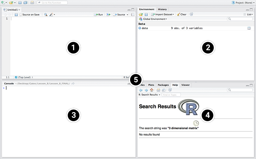
RStudio Layout
- Script Window: In this window, collections of commands (scripts) can be edited and saved. If this window is not present upon opening RStudio, you can open it by clicking File→New File→R Script. Just typing a command in the Script window and clicking enter will not cause R to run the command; the command has to get entered in the Console window before R executes the command. If you want to run a line from the script window, you can click Run on the toolbar or press CTRL+ENTER to enter the line into the console view.
- Environment / History Window: Under the Environment tab you can see which data and values R has in its memory. The History tab shows what has been entered into the console.
- Console window: Here you can type simple commands after the > prompt and R will then execute your command. This is the most important window, because this is where R actually runs commands.
- Files / Plots / Packages / Help: Here you can open files, view plots (also previous plots), install and load packages or use the help function.
- You can change the size of each of the windows by dragging the grey bars between the windows.
Working Directory
Your working directory is a folder on your computer from where files can be entered, or read, into R. When you ask R to open a file with a read command, R will look in the working directory folder for the specified file. When you tell R to save a data set or figure which you’ve created, R will also save the data or figure as a file in the same working directory folder.
Set your working directory to a folder where all of the example data files for this lesson are located.
- Create a folder on your desktop; for this example the folder will be called wd. Then, obtain the default working directory by entering the command getwd() into the console window. R returns the default working directory below.
getwd()
[1] “C:/Users/<Username>/Documents”
- Next, set the working directory to the folder on your desktop, wd, using the setwd() command in the Console window:
setwd(“C:/Users/<Username>/Desktop/wd”)
Notice that to set our working directory to a folder on our desktop, we enter everything that was returned by R from the getwd()command before the word Documents, change Documents to Desktop, then add a forward slash followed by the name of our folder (wd).
Make sure that the slashes are forward slashes and that you don’t forget the quotation marks. R is case sensitive, so make sure you write capitals where necessary. Within the RStudio interface you can also go to Session → Set working directory to select a folder to be your working directory.
Libraries
R can do many kinds of statistical and data analyses. The analyses methods are organized in so-called packages. With the standard installation, most common packages are installed. To get a list of all installed packages, go to the packages window (lower right in RStudio). If the box in front of the package name is ticked, the package is loaded (activated) and can be used. You can also type library() in the console window to view the loaded packages.
There are many more packages available on the R-website. If you want to install and use a package (for example, the package called “geometry”) you should:
- Install the package: click on the “packages” tab at the top of the lower-right window in RStudio. Click “install”, and in the text box under the heading “packages”, type “geometry”. You can also simply enter install.packages(”geometry”) in the console window to install the package.
- Load the package: under the “packages” tab at the top of the lower-right window in RStudio, check the boxes of the packages you wish to load (i.e. “geometry”). You can also simply type library(”geometry”) in the console window to load the package.
Getting Help in R
If you know the name of the function you want help with, you can just type a question mark followed by the name of the function in the console window. For example, to get help on aov, just enter:
?aov
Sometimes you don’t know the exact name of a function, but you know the subject on which you want help (i.e., Analysis of Variance). The simplest way to get help in R is to click the “Help” tab on the toolbar at the top of the bottom-right window in RStudio, then enter the subject or function that you want help within the search box at the right. This will return a list of help pages pertaining to your query.
Another way to obtain the same list of help pages is by entering the help.search command in the Console. The subject or function which you’d like information about is put inside of brackets and quotation marks, directly following the help.search command. For example, to obtain information about Analysis of Variance, enter into the console:
help.search(“Analysis of Variance”)
If you’d like to see an example of how a function is used, enter “example” followed by the function that you’d like to see an example of (within quotation marks and brackets). For instance, if we wanted to see an example of how the aov function can be used, we can enter into the console:
example(“aov”)
An example is returned in the console window.
Reading the CSV File
Now, we want to read the CSV file from our working directory into RStudio. At this point, we learn an important operator: <-. This operator is used to name data that is being read into the R data frame. The name you give to the file goes on the left side of this operator, while the command read.csv goes to its right. The name of the CSV file from your working directory is entered in the parenthesis and within quotations after the read.csv command. The command header = T is used in the function to tell R that the first row of the data file contains column names, and not data.
Read the file into R by entering into the Console:
data <- read.csv(“Review Models Install R ALA data.csv”, header = T)
Tip: If you are working out of the Console and received an error message because you typed something incorrectly, just press the ↑ key to bring up the line which you previously entered. You can then make corrections on the line of code without having to retype the entire line in the console window again. This can be an extremely useful and time saving tool when learning to use a new function. Try it out.
If the data was successfully read into R, you will see the name that you assigned the data in the Workspace/History window (top-right).
Examining the Data
Let us look at the first few rows of the data. We can do this by entering the command head(data) in the console. If we want to look at a specific number of rows, let us say just the first 3 rows, we can enter head(data, n=3) in the Console. Try both ways.
First, enter into the console:
head(data)
Pop Rep Yield
1 30 1 137.1
2 30 2 124.4
3 30 3 145.9
4 40 1 166.1
5 40 2 147.4
6 40 3 142.7
Now, try looking at only the first 3 rows:
head(data)
Pop Rep Yield
1 30 1 137.1
2 30 2 124.4
3 30 3 145.9
Viewing and Removing Datasets
Now, let us say we are finished using this dataset and want to remove it from the R data frame. To accomplish this, we can use the rm command followed by the name of what we want removed in parenthesis. Let us remove the data from the R data frame. Enter into the console rm(data).
rm(data)
The dataset data should no longer be present in the Workspace/History window.
What if we have many things entered in the R data frame and want to remove them all? There are two ways that we can do this. To demonstrate how, let us first enter 3 variables (x,y, and z) into the R data frame. Set x equal to 1, y equal to 2, and z equal to 3.
x<-1
y<-2
z<-3
Clicking on ‘clear’ in the History/Environment window (top right) will clear everything in the R data frame. Another way to remove all data from the R data frame is to enter in the console:
rm(list=1s())
Try both ways.
EDA with R
Objectives
- Students will conduct exploratory data analyses (EDA) on data from a simple Completely Randomized Design (CRD).
- Assess whether students know how to interpret results from EDA.
- Students will conduct an Analysis of Variance (ANOVA) on data from a simple CRD.
Directory Of R Commands Used
- getwd()
- setwd()
- read.csv()
- rm()
- rm(list=())
- hist()
- attach()
- boxplot()
- str()
- as.factor()
- aov()
- summary()
Set Working Directory
Before you can conduct any analysis on data from a text file or spreadsheet, you must first enter, or read, the data file into the R data frame. For this activity, our data is in the form of an Excel comma separated values (or CSV) file; a commonly used file type for inputting and exporting data from R.
Make sure that the data file for this exercise is in the working directory folder on your desktop.
Note: We previously discussed how to set the working directory to a folder named on your desktop. For this activity, we will repeat the steps of setting the working directory to reinforce the concept.
In the Console window, enter getwd(). R will return the current working directory below the command you entered:
getwd()
[1] “C:/Users/<Username>/Documents”
Set the working directory to the folder on your desktop by entering setwd(). For a folder named ‘wd’ on our desktop, we enter:
setwd(“C:/Users/<Username>/Desktop/wd”)
Please note that the working directory can be in any other folder as well, but the data file has to be in that specific folder.
Reading the CSV File
Now, we want to read the CSV file from our working directory into RStudio. At this point, we learn an important operator: <-. This operator is used to name data that is being read into the R data frame. The name you give to the file goes on the left side of this operator, while the command read.csv goes to its right. The name of the CSV file from your working directory, in this case CRD.1.data.csv, is entered in the parenthesis and within quotations after the read.csv command. The command header = T is used in the function to tell R that the first row of the data file contains column names, and not data.
data <- read.csv(“CRD.1.data.csv“, header = T)
Tip: If you are working out of the Console and received an error message because you typed something incorrectly, just press the ↑ key to bring up the line which you previously entered. You can then make corrections on the line of code without having to retype the entire line in the console window again. This can be an extremely useful and time saving tool when learning to use a new function. Try it out.
If the data was successfully read into R, you will see the name that you assigned the data in the Workspace/History window (top-right).
Exploring the Data
Let us do some preliminary exploring of the data.
Read the data set into the R data frame.
data <- read.csv(“CRD.1.data.csv“, header = T)
First, let us look at a histogram of the yield data to see if they follow a normal distribution. We can accomplish this using the hist command.
Enter into the console:
hist(data$Yield, col=”blue”, main= “Histogram of Yield of 3 Synthetic Maize Populations”,
xlab=”Yield (bushels/acre)”, ylab=”Frequency”)
R returns the histogram in the Files/Plots/Packages/Help window (bottom-right).
Histogram
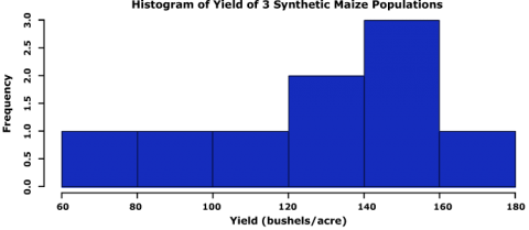
Let us go through the command we just entered: data$Yield specifies that we want to plot the values from the column Yield in the data, col=”blue” indicates which color the histogram should be, the entry in quotations after main= indicates the title that you’d like to give the histogram, the entries after xlab= and ylab= indicate how the x and y axes of the histogram should be labeled. The histogram appears in the bottom-right window in RStudio.
The histogram can be saved to your current working directory by clicking ‘export’ on the toolbar at the top of the lower-right window, then clicking “save plot as PNG” or “save plot as a PDF”. You may then select the size dimensions you would like applied to the saved histogram.
Boxplots
Let us now look at some boxplots of yield by population for this data. First, enter into the Console window attach(data). The attach command specifies to R which data set we want to work with, and simplifies some of the coding by allowing us just to use the names of columns in the data, i.e. Yield vs. data$Yield. After we enter the attach command, we’ll enter the boxplot command.
attach(data)
boxplot(Yield~Pop, col=”red”, main=”Yield by Population”, xlab=”Synthetic Population”,
ylab=”Yield”)
R returns the boxplot in the bottom-right window.
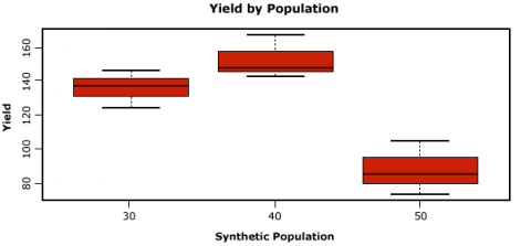
Let us go through the boxplot command: Yield~Pop indicates that we want boxplots of the yield data for each of the 3 populations in our data, col= indicates the color that we want our boxplots to be, main= indicates the title we want to give the boxplots, and xlab= and ylab= indicate what we want the x and y axes labeled as.
Note: Yield is capitalized in our data file, thus it MUST also be capitalized in the boxplot command.
Mean and Coefficient of Variance
The coefficient of variance can be calculated for each population in the data set. Looking at the data, we can see that lines 1 to 3 pertain to population 30. We know that the coefficient of variation for a sample is the mean of the sample divided by the standard deviation of the sample. By using the command mean(), we can calculate the mean for a sample. Remember that to specify a column from a data frame, we use the $ operator. If we want to calculate the mean of population 30 from the data (rows 1 to 3 in the data), we can enter
mean(data$Yield[1:3])
To calculate the standard deviation of the yield for population 30, enter
sd(data$Yield[1:3])
The coefficient of variance is therefore calculated by entering
mean(data$Yield[1:3])/sd(data$Yield[1:3])
One-Factor ANOVA of a CRD
Now that we’ve gained some intuition about how the data behave, let us carry out an ANOVA with one factor (Pop) on the data. We first need to specify to R that we want Population to be a factor. Enter into the Console
Pop<-as.factor(Pop)
Let us go through the command above: as.factor(data$Pop) specifies that we want the Pop column in dataset data to be a factor, which we’ve called Pop.
Now that we have population as a factor, we’re ready to conduct the ANOVA. The model that we are using for this one-factor ANOVA is Yield=Population.
In the Console, enter
mean(data$Yield[1:3])/sd(data$Yield[1:3])
Interpret the Results
Let us look at the ANOVA table. Enter out in the Console window.
out
In this ANOVA table, the error row is labelled Residuals. In the second and subsequent columns you see the degrees of freedom for Pop and Residuals (2 and 6), the treatment and error sums of squares (6440 and 1011), the treatment mean square of 3220, the error variance = 169, the F ratio and the P value (19.1 and 0.0025). The double asterisks (**) next to the P value indicate that the difference between the yield means of the three populations is significant at 0.1% (i.e. we reject the null hypothesis that the yield means of each population are statistically equivalent). Notice that R does not print the bottom row of the ANOVA table showing the total sum of squares and total degrees of freedom.
Hypothesis Tests
Objectives
Demonstrate ability to interpret types of errors that can be made from testing various kinds of hypotheses.
Statistical Inference
The purpose of statistical inference is to interpret the data we obtain from sampling or designed experiments. Preliminary insights come from graphical data summaries such as bar charts, histograms, box plots, stem-leaf plots and simple descriptive statistics such as the range (maximum, minimum), quartiles, and the sample average, median, mode. These exploratory data analysis (EDA) techniques should always be used prior to estimation and hypothesis testing. However, prior to conducting EDA, the phenotype should be modeled using the parameters in the experimental and sampling designs.
Null and Alternative Hypotheses
Hypotheses are questions about parameters in models. For example, “Is the average value for a trait different than zero?” is a question about whether the parameter µ is non-zero. Formally, the proposition [latex]H_0 : \mu = 0[/latex], is called the null hypothesis, while a proposition [latex]H_{\alpha} : \mu \neq 0[/latex] is called an alternative hypothesis.
A test statistic is used to quantify the plausibility of the data if the null hypothesis is true. For this simple hypothesis the value of the test statistic should be close to zero if the null hypothesis is true and far from zero if the alternative hypothesis is true. Notice that in all linear models there is a parameter, ε, included to indicate that there is some random variability in the data that cannot be ascribed to the other parameters in the model. It is entirely possible that the variability in the data is due entirely to ε and that an estimate of µ that is not zero is due to this random variability.
Inferential Errors from Hypothesis Testing
How often will the estimate of µ be different from zero when Ho is true? We can answer this question by rerunning an experiment in which we know µ = 0 a million times, generate a histogram of the resulting distribution and then see how often (relative to 1 million) an estimated mean that is equal to or more extreme than our experimental estimate occurs. This is the frequency associated with finding our estimated value or a more extreme value when Ho is true.
The good news is that we don’t have to conduct a million such experiments because someone else has already determined the distribution when µ = 0, is true. The frequency value associated with a test statistic as extreme or more extreme than the one observed is often referred to as a ‘p’ value. The smaller the p value, the more comfortable we should be in rejecting the null hypothesis in favor of an alternative hypothesis. Keep in mind that we can be wrong with making such a decision. In fact we are admitting that such a decision will be incorrect at a frequency of p.
Error Types
Consider another simple example where we hypothesize that two genotypes have the same mean for some trait of interest. The difference between two genotypes is tested by Equation 19:
[latex]\delta_{ij} = g_i - g_j[/latex]
[latex]\textrm{Equation 19}[/latex] Formula for testing the difference between two genotypes.
where:
[latex]g_i\; and\; g_j[/latex] = the ith and jth true genotypic effects on the trait of interest.
Whether or not a decision based on observed data is correct depends on the true value of the difference between the means (Table 4).
| Decision based on empirical data | True Situation | ||
| [latex]\delta_{ij} 0[/latex] | [latex]\delta_{ij} = 0[/latex] | [latex]\delta_{ij} > 0[/latex] | |
| 1. [latex]\delta_{ij} 0[/latex] | Correct decision | Type I error | Type III error |
| 2. [latex]\delta_{ij} = 0[/latex] | Type II error | Correct decision | Type II error |
| 3. [latex]\delta_{ij} >[/latex] | Type III error | Type I error | Correct decision |
A Type I error is committed if the null hypothesis is rejected when it is true (δij=0 and the hypothesis of equality is rejected). A Type II error is committed if the null hypothesis is accepted when it is really false (δij≠0 and the hypothesis of equality is not rejected). Type I error is also called “false positive”, and Type II error is also known as a “false negative.” A Type III error occurs if the first decision is made when the third decision should have been made. This error also occurs if the third decision was made when the first decision was correct. Type III errors are sometimes called reverse decisions.
Significance Levels
The probability (or frequency) of a Type I error is the level of significance, denoted by [latex]\alpha[/latex].
The choice of [latex]\alpha[/latex] can be any desirable value between 0 and 1.
For example, if a test is carried out at the 5% level, [latex]\alpha[/latex] is 0.05.
If you carry out tests at 5% level you will reject 5% of the hypotheses you test when they are really true.
The rejection rate can be reduced by choosing a lower level of [latex]\alpha[/latex]
However, the choice of [latex]\alpha[/latex] will affect the frequency of Type II and Type III errors.
A Type III error rate, γ, is the frequency of incorrect reverse decisions and is always less than α/2 even for the smallest magnitudes of the standardized true difference, δij/σd where σd is the parameter value of the standard error of the mean difference. Representative values of γ are shown below in Table 5.
| Standardized true difference [latex]\delta_{ij}/\sigma_d[/latex] | Significance Level ([latex]\alpha[/latex]) | |||
| 0.05 | 0.10 | 0.20 | 0.40 | |
| 0.3 | 0.0127 | 0.0271 | 0.0584 | 0.1283 |
| 0.9 | 0.002 | 00068 | 0.0167 | 0.0438 |
| 1.5 | 0.0005 | 0.0014 | 0.0039 | 0.019 |
| 2.1 | 0.0001 | 0.0002 | 0.0008 | 0.0026 |
| 2.7 | 0.0000 | 0.0000 | 0.0001 | 0.0005 |
Power of the Test
Lastly, consider the error that is committed if the null hypothesis is not rejected when it is truly false. This is also known as a Type II error, and the probability of this type of error is denoted by β. It is the frequency of failure to detect real differences and is also affected by both the choice of α and the magnitude of the standardized true difference (Table 6).
| Standardized true difference [latex]\delta_{ij}/\sigma_d[/latex] | Significance Level [latex]\alpha[/latex] | |||
| 0.05 | 0.10 | 0.20 | 0.40 | |
| 0.3 | 0.941 | 0.886 | 0.781 | 0.579 |
| 0.9 | 0.863 | 0.774 | 0.639 | 0.437 |
| 1.5 | 0.697 | 0.571 | 0.419 | 0.248 |
| 2.1 | 0.469 | 0.340 | 0.214 | 0.107 |
| 2.7 | 0.251 | 0.158 | 0.085 | 0.035 |
Notice that α + β ≠ 1.0. The power of the test is = 1 – β and is denoted π, thus β + π = 1.0. The power of a test is the probability of rejecting the null hypothesis when it is false. It can be increased by decreasing either the value of α or decreasing the value of σd by increasing the number of replications per treatment or by improving the experimental design.
Analysis of Variance
Objectives
Students will demonstrate the ability to conduct and interpret Analysis of Variance.
Statistical Inference
The purpose of statistical inference is to interpret the data we obtain from sampling or designed experiments. Preliminary insights come from graphical data summaries such as bar charts, histograms, box plots, stem-leaf plots, and simple descriptive statistics such as the range (maximum, minimum), quartiles, and the sample average, median, mode. These exploratory data analysis (EDA) techniques should always be used prior to estimation and hypothesis testing. However, prior to conducting EDA, the phenotype should be modeled using the parameters in the experimental and sampling designs.
Background
The AOV has been the primary tool for testing hypotheses about parameters in linear models. The AOV was originally developed and introduced for analyses of quantitative genetic questions by R.A. Fisher (1925). Since its introduction, the assumptions underlying the AOV have guided development of sophisticated experimental designs, and with increasing computational capabilities the AOV has evolved to provide estimates of variance components from these designs. While the breadth and depth of experimental design and analyses of linear models are beyond the scope of this class, it is worth recalling the salient features of experimental design and their impact on inferences from the AOV.
Experimental Designs consist of design structures, treatment structures, and allocation of these structures to experimental units. Typical design structures utilized by plant breeders include Randomized Complete Block, Lattice Incomplete Block and Augmented Designs. The primary treatment designs of interest of plant breeders involve allocation of genotypes to experimental units. This is accomplished primarily through mating, although with the emergence of biotechnologies, such as protoplast fusion, tissue culture and various transgenic technologies, there are many ways to allocate treatments (genotypes) to experimental units. Would you consider treatments from these technologies as fixed or random effects? Why? Experimental units can be split in both time and space, resulting in the ability to apply treatment and design structures to different sized experimental units.
Design Principles
Design principles in allocation of treatment and design structures to experimental units include Randomization, Replication and Blocking. These are principles rather than rigid rules. As such, they provide flexibility in designing experiments to draw inferences about biological questions. Assuming that these principles are applied appropriately, experimental data can be used for obtaining unbiased estimates of treatment effects, variances, covariances, and even predict breeding values.
Completely Random Design
Let us imagine that we have two plant introduction accessions. We wish to evaluate whether these two accessions are unique with respect to yield.
Assume that we have 10 plots available for purposes of testing the null hypothesis that there is no difference in their yield. Also, assume that we have enough seed to plant 200 seeds in each plot.
Let us next assume that the 10 plots consist of two-row plots that are arranged in a 5×2 grid consisting of five ranges with 2 plots per range. We can randomly assign seed from each accession to the 10 plots. This would represent a Completely Random Design (CRD). Can you explain why?
Fixed and Random Effects
Prior to execution of the experiment, we want to model the phenotypic data using a linear function. In this case we would model the phenotypic data using Equation 20:
[latex]Y_{ij} = \mu_{i} + \varepsilon_{ij}[/latex]
[latex]\textrm{Equation 20}[/latex] Linear model for phenotype.
where:
[latex]Y_{ij}[/latex] = the yield of plot i, j, where i = 1, 2 for accession and j = 1, …, 5 for replicate,
[latex]\mu_{i}[/latex] = represents the mean of accession i,
[latex]\varepsilon_{ij}[/latex] = the error, ~ i.i.d. N(0, σ2).
It is important to get in the habit of recognizing whether the parameters of the model are considered random or fixed effects.
In this first model, since we selected the two accessions, rather than sampled them from some population, we should consider them to be fixed effects. The parameter εi,j representing the residual or error in the model is based on a sample of plots to which experimental units are assigned, so εi,j is considered a random effect.
AOV Based on Yield
Next, let us say that we evaluate the plots for yield (bushels per acre) as well as stand counts (plants per plot) at the time of harvest. The resulting data might look something like in Table7.
| n/a | PI accession 1 | PI accession 2 | ||
| Block | (t/ha) | (plants/plot) | (t/ha) | (plants/plot) |
| 1 | 1.69 | 91 | 1.88 | 102 |
| 2 | 1.95 | 122 | 1.82 | 89 |
| 3 | 2.20 | 143 | 2.01 | 139 |
| 4 | 2.13 | 145 | 2.01 | 147 |
| 5 | 1.76 | 110 | 1.95 | 112 |
If we conduct an AOV based on yield using the model for a CRD, we will generate a table that looks something like Table 8.
| Source | df | MS | F | Prob |
| Accession | 1 | n/a | n/a | n/a |
| Residual | 8 | n/a | n/a | n/a |
Blocking Ranges
Suppose that we suspect a gradient for some soil factor (moisture, organic matter, fertility, etc.) across the ranges. In order to remove the effect of the gradient on our comparisons between the two accessions, we should probably ‘block’ each range as a factor in our model.
Let us further assume that we block the accession ‘treatments’ into five blocks consisting of two plots each. If we randomly group pairs of the accessions into 5 sets, next randomly assign each set to a range, and third, randomly assign each accession within a set to the plots within ranges, we will have a randomized complete block design (RCBD) that can be modeled as [latex]Y_{ij} = b_{j} + \mu_{i}+\epsilon_{ij}[/latex] where the definition of parameters is the same as the CRD model, but with the added term for a blocking factor.
Mixed Linear Model
In this second model, the accessions are selected so we should consider them to be fixed effect parameters. Although the block parameter represents a sample of many possible blocks in the field trial, there are only a few blocks that represent a “nuisance” source of variability, so we can treat them as a fixed effect, while the parameter εij represents the residual or error in the model which is based on a sample of plots to which experimental units are assigned.
Thus εij is considered random effects where εij ~ i.i.d. N(0, σe2), and the model is considered a mixed linear model.
| Source | df | MS | F | Prob |
| Block | 4 | n/a | n/a | n/a |
| Accession | 1 | n/a | n/a | n/a |
| Residual | 4 | n/a | n/a | n/a |
Regression and Prediction
Objectives
Demonstrate ability to conduct and interpret regression analyses.
Statistical Inference
The purpose of statistical inference is to interpret the data we obtain from sampling or designed experiments. Preliminary insights come from graphical data summaries such as bar charts, histograms, box plots, stem-leaf plots, and simple descriptive statistics such as the range (maximum, minimum), quartiles, and the sample average, median, mode. These exploratory data analysis (EDA) techniques should always be used prior to estimation and hypothesis testing. However, prior to conducting EDA, the phenotype should be modeled using the parameters in the experimental and sampling designs.
Linear Regression
Historically, linear (and non-linear) regression has not been utilized extensively by plant breeders, although it provides the conceptual foundation for understanding additive genetic models and analysis of covariance. Recently, with the emergence of molecular marker technologies, the importance of linear regression has manifested itself in the development of predictive methods such as Genomic Prediction. Linear regression is an approach to modeling the relationship between a scalar dependent variable Y (e.g., harvestable grain yield per unit of land) and one or more explanatory variables (e.g., breeding values of lines involved in crosses) denoted by X.
Basic Assumptions
In linear regression, the phenotype is modeled using a linear function. There are four basic assumptions made about the relationship between a response variable Y and an explanatory variable X.
- All Y values are from independent experimental or sample units.
- For each value of X, the possible Y values are distributed as normal random variables.
- The normal distribution for Y values corresponding to a particular value of X has a mean μ{Y|X} that lies on a line (Equation 21):
[latex]µ{\{Y|X\}} = \beta_0 + \beta_1X[/latex]
[latex]\textrm{Equation 21}[/latex] Formula for estimating the mean.
where:
[latex]β_{0}[/latex] = the intercept and represents the mean of the Y values when X = 0,
[latex]β_{1}[/latex] = the slope of the line, that is, the change in the mean of Y per unit increase in X.
- The distribution of Y values corresponding to a particular value of X has standard deviation σ {Y|X). The standard deviation is usually assumed to be the same for all values of X so that we may write σ{Y|X}=σ. Violation of the last assumption is typical in plant breeding data and the development of methods to account for unequal variances is an area of important research.
Simple Linear Regression
Suppose we have n observations of a response variable Y and an explanatory variable X: (X1,Y1), . . . , (Xn,Yn). The model can be rewritten as in Equation 22:
[latex]Y_i = \beta_0+ \beta_1X_1 + e_i[/latex]
[latex]\textrm{Equation 22}[/latex] Linear model for phenotype.
where:
[latex]\textrm{\small All terms}[/latex] are as defined previously,
for i = 1, . . . , n experimental units. ei , . . . , en are assumed to be independent normal random variables with mean 0 and standard deviation σ{Y|X}=σ. Thus, least-squares estimates of the Yi values are obtained using Equation 23:
[latex]\hat{Y}_i = \hat{\beta}_0 + \hat{\beta}_{i}x_i[/latex]
[latex]\textrm{Equation 23}[/latex] Least squares estimates model for Y values.
where:
[latex]\textrm{\small All terms}[/latex] are as defined previously.
The residual ei (e1, . . . , en) can be calculated as represented in Equation 24:
[latex]\hat e_i = Y_i -\hat{Y}_i = Y_i - (\hat{\beta}_0 + \hat{\beta}_{i}x_i)[/latex]
[latex]\textrm{Equation 24}[/latex] Formula for estimating residuals.
where:
[latex]\textrm{\small All terms}[/latex] are as defined previously.
Parameter Estimates
The estimators for parameters [latex]\beta_0[/latex], [latex]\beta_i[/latex] , and σ are
[latex]\eqalign{\hat{\beta}_i &= \frac{\sum^n_{i-1}{(x_i-\bar{x})}{(y_i-\bar{y})}}{\sum^n_{i=1}{{(x_i-\bar{x})}^2}}\\ \hat{\beta}_0 &= \bar{Y} - \hat{\beta_1}{(\bar{x})}\\ \hat{\sigma} &= \sqrt{\frac{\sum^n_{i=1}{(Y_i - \hat{Y})}^2}{n-2}} }[/latex]
Prediction
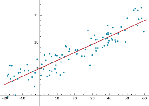
Notice that Equation 23, [latex]\hat{Y}_i = \hat{\beta_0} + \hat{\beta}_ix_i[/latex], provides a predicted value of Yi. Imagine that the xi (i=1, …, n) values are a genotypic index for cultivar/individual i, such as the sum of all allelic values (+1 or -1) at quantitative trait loci throughout the genome. Some cultivars could have 60 positive allelic values and no negative allelic values, while other cultivars could have a genotypic index of -20 (see Figure 10). If the positive genotypic index values are associated with high phenotypic values, such as in the figure, then we will have a strong positive linear relationship between the genotypic index and the phenotypes. A strong linear relationship can enable the plant breeder to predict phenotypes without having to spend resources on growing cultivars. The stronger the linear relationship is between the genotypic index and the phenotype (less variability around the line), the better the ability to predict. This concept represents the foundation for what is widely referred to as Genomic Prediction.
There are a number of details about how allelic values are estimated and combined into genotypic indices. The foundational concepts that address these details are covered in the Introduction to Quantitative Genetics section.
Analysis of Covariance
Objective: Demonstrate ability to conduct and interpret Analysis of Covariance
Statistical Inference
The purpose of statistical inference is to interpret the data we obtain from sampling or designed experiments. Preliminary insights come from graphical data summaries such as bar charts, histograms, box plots, stem-leaf plots, and simple descriptive statistics such as the range (maximum, minimum), quartiles, and the sample average, median, mode. These exploratory data analysis (EDA) techniques should always be used prior to estimation and hypothesis testing. However, prior to conducting EDA, the phenotype should be modeled using the parameters in the experimental and sampling designs.
AOC is typically applied when there is a need to adjust results for variables that cannot be controlled by the experimenter. For example, imagine that we have two plant introduction accessions and we wish to evaluate whether these two accessions are unique with respect to yield. Also, imagine that germination rates for each accession is different but unknown, especially under field conditions in a new environment. We could decide to overplant each plot and reduce the number of plants per plot to a constant number equal to a stand count that is typical under current Agronomic practices. However, such an approach will be labor-intensive and not as informative as simply adjusting plot yields for stand counts.
Example
Assume that we have 10 plots available for purposes of testing the null hypothesis that there is no difference in their yield. Also, assume that we have enough seed to plant 200 seeds in each plot, although current agronomic practices are more closely aligned with stands of about 125 plants per plot. Let us next assume that the 10 plots consist of two-row plots that are arranged in a 5×2 grid consisting of five ranges with 2 plots per range. Suppose that we suspect a gradient of some soil factor (moisture, organic matter, fertility, etc.) across the ranges. In order to remove the effect of the gradient on our comparisons between the two accessions we should probably ‘block’ each range as a factor in our model. If we randomly group pairs of the accessions into 5 sets, next randomly assign each set to a range and third randomly assign each accession within a set to the plots within ranges, we will have a RCBD. At the time of harvest, we evaluate the plots for yield (bushels per acre) as well as stand counts (plants per plot). The resulting data are arranged in Table 10.
| n/a | PI accession 1 | PI accession 2 | ||
| Block | (t/ha) | (plants/plot) | (t/ha) | (plats/plot) |
| 1 | 1.69 | 91 | 1.88 | 102 |
| 2 | 1.95 | 122 | 1.82 | 89 |
| 3 | 2.20 | 143 | 2.01 | 139 |
| 4 | 2.13 | 145 | 2.01 | 147 |
| 5 | 1.76 | 110 | 1.95 | 112 |
Model Equation
If we model the yield data as Yij = bj + µi+ εij , where Yij is the yield of plot ij , µi represents the mean of accession i, bj represents the jth block in which each pair of accessions are grown and εij ~ i.i.d. N(0,σ2), the resulting analysis revealed that the variability between accessions is not much greater than the residual variability. We might interpret this to mean that there is no difference in yield between the two accessions. However, our real interest is in whether there is a difference between the accessions at the same stand counts. A more appropriate model for the question of interest is as in Equation 25:
[latex]Y_{ij} = \alpha_i + \beta_iX_{ij} + b_j + \varepsilon_{ij}[/latex]
[latex]\textrm{Equation 25}[/latex] Formula for calculating phenotype in a plot.
where:
[latex]\alpha_i[/latex] = intercept for accession i,
[latex]\beta_i[/latex] = slope of accession i,
[latex]X_{ij}[/latex] = the jth stand count in accession i (i = 1, 2,)
[latex]b_{j}[/latex] = random effect parameter.
The model has two intercepts, denoted αi (i = 1, 2) for each of the accessions, and two slopes denoted ßi (i = 1, 2), for each of the accessions. Xij is the jth stand count in accession i (i = 1, 2). The model also has random effects parameters denoted by bj and εi,j where bj~ i.i.d. N(0,σb2) and εi,j ~ i.i.d. N(0, σe2). The resulting analyses of variability associated with each of the parameters is known as Analysis of Covariance, and can be thought of as an approach that takes advantage of both regression and ANOVA, i.e., an AOC model includes parameters representing both regression and factor variables. The result of the estimation procedure will enable us to evaluate whether the accessions are equal at stand counts of interest. In other words it will be possible to adjust yield values to various stand counts of interest. As a matter of ethics in science, the variable stand count of interest needs to be modeled prior to conducting the field trial.
Computational Considerations
Key Concepts
As long as data are balanced all computational algorithms will provide the same estimates of variance components.
- When data are not balanced, either by design or accident, simple algorithms implemented in many widely used software packages (EXCEL, JMP for exampes) will not provide correct estimates of variance components.
Statistical Inference
The purpose of statistical inference is to interpret the data we obtain from sampling or designed experiments. Preliminary insights come from graphical data summaries such as bar charts, histograms, box plots, stem-leaf plots and simple descriptive statistics such as the range (maximum, minimum), quartiles, and the sample average, median, mode. These exploratory data analysis (EDA) techniques should always be used prior to estimation and hypothesis testing. However, prior to conducting EDA, the phenotype should be modeled using the parameters in the experimental and sampling designs.
Computational Methods
Most plant breeding data are obtained using a limited number of field plot designs consisting of lines (cultivars, hybrids, synthetics, etc.), environments and occasionally complete blocks, but usually incomplete blocks, within environments. Further, numbers of observations per source of variation are seldom balanced; even if designed for balance, some plots are lost during the course of a growing season. Thus, while the algorithm for obtaining EMS (described in the section Statistical Inference: Analysis of Variance) is useful for learning basic concepts, it is of little practical use for most plant breeding projects. Just as the estimates of means need to be adjusted through use of lsmeans, advanced computational methods are needed to obtain accurate estimates of variance components of the linear model when data are obtained from unbalanced conditions. The computational methods are affected by fixed effects, random effects or a mixture of both types of effects. There are three primary computation methods for estimating variance components: Method of Moments (MM), Maximum Likelihood (ML), and Restricted Maximum Likelihood (REML).
Regression, Anova, and AOC
Computation of the MM estimators of variance components is essentially a matter of equating observed mean squares, calculated using the sums of squared deviations and cross products, with the expected mean squares, as demonstrated by Lorenzen and Anderson (1993, Design of Experiments: A No-Name Approach. p 71-72). These are appropriate if the data are balanced. Most advanced statistical software packages, e.g., SAS and R, calculate the sums of squares and cross products for the MM using the MIVQUE(0) algorithm (Minimum Variance Quadratic Unbiased Estimator, with no weighting for random effects).
Computation of ML and REML are derived from MIVQUE(0); both use MIVQUE(0) estimates as starting points in an iterative algorithm that maximizes the likelihood function, assuming that the random effects are distributed as random normal variables. The difference between ML and REML is that the likelihood function in REML is maximized only for the random effects, i.e., the fixed effects are removed from the likelihood function. For a model consisting of only random effects, both ML and REML will provide the same results. Indeed, for completely balanced data from random effects models, all three computational methods provide the same results. When dealing with unbalanced data or mixed effect models, REML has been shown to be the best computational method.
Further Considerations
As a practical matter, if your data is missing less than 10% of the experimental units within any environment, the MM approach will provide estimates that are almost as good as REML. Otherwise, the estimates should be obtained with mixed model equations (MME) and a REML algorithm. We encourage the use of R or SAS software for conducting data analyses. R is free, while the SAS license fees pay for more rigorous quality assurance.
Matrix Algebra
A matrix is a collection of numerical values arranged in rows and columns. Herein, the elements of a matrix are enclosed in brackets. For example,
[latex]A = \begin{bmatrix} &a_{11} &a_{12} \\ &a_{21} &a_{22} \end{bmatrix}[/latex].
is a matrix with 4 elements arranged in 2 rows and two columns.
Matrices with more than two or more rows and columns are denoted with upper case bold letters. Vectors are a special type of matrix with only one row or one column. For example,
[latex]x = \begin{bmatrix} &x_1 \\ &x_2 \\ &x_3 \\ &x_4 \\ &x_5 \end{bmatrix}\space or \space y = \begin{bmatrix} &y_1 &y_2 &y_3 \end{bmatrix}[/latex].
Special Kinds of Matrices
Vector matrices are denoted with lower case bold italicized letters. A matrix consisting of only one row and one column is referred to as a scalar matrix. A square matrix has the same number of rows and columns. A diagonal matrix is a square matrix with off-diagonal elements equal to 0. An identity matrix is a diagonal matrix with diagonal elements = 1. The identity matrix is almost always denoted I.
Operations
Matrices must be conformable, i.e., matrix operations have requirements on the numbers of rows and columns.
It is possible to add or subtract two matrices, but only if they have the same numbers of rows and columns. For example,
[latex]C = A -B = \begin{bmatrix} &c_{11} &c_{12} &c_{13} \\ &c_{21} &c_{22} &c_{23} \\ &c_{31} &c_{32} &c_{33} \end{bmatrix} = \begin{bmatrix} &{a_{11}-b_{11}} &{a_{12} - b_{12}} &{a_{13}-b_{13}} \\ &{a_{21}-b_{21}} &{a_{22} - b_{22}} &{a_{23}-b_{23}} \\ &{a_{31} - b_{31}} &{a_{32}-b_{32}} &{a_{33}- b_{33}} \end{bmatrix}[/latex].
It is possible to multiply a matrix by a scalar value (say ‘v’) by simply multiplying all elements of the matrix by the scalar value, v. Thus,
[latex]D = vA =Av = D = \begin{bmatrix} &va_{11} &va_{12} &va_{13} \\ &va_{21} &va_{22} &va_{23} \\ &va_{31} &va_{32} &va_{33} \end{bmatrix}[/latex].
Multiplying Vectors
It is possible to multiply two vectors, but only if 1) one of the vectors is a row vector, 2) the second is a column vector, 3) the row vector has as many elements as the column vector. For example,
[latex]\begin{bmatrix} 1 & 3 & 5 \end{bmatrix} \begin{bmatrix} 2\\ 4\\ 6 \end{bmatrix}\space is\space a\space legal\space operation,\space whereas\space \begin{bmatrix} 1 & 3 \end{bmatrix} \begin{bmatrix} 2\\ 4\\ 6 \end{bmatrix}\space is\space not[/latex].
The operation of vector multiplication in the first instance indicates that we have a 1×3 matrix multiplied by a 3×1 matrix. The way we carry out the vector multiplication is to multiply the elements from each matrix in a pairwise manner, then sum the results of all 3 pairs:
[latex]\begin{bmatrix} &1 &3 &5 \end{bmatrix}\begin{bmatrix} &2\\ &4\\ &6 \end{bmatrix} = 1 \times 2 + 3 \times 4 + 5 \times 6 = 44[/latex].
Multiplying Vectors In Reverse
We could also apply the rule of multiplying and summing pairs of elements to the reverse arrangement of these two vectors:
[latex]\begin{bmatrix} &2\\ &4\\ &6 \end{bmatrix}\begin{bmatrix} &1 &3 &5 \end{bmatrix} = \begin{bmatrix} &2 &4 &6 \\&4 &12 &20 \\&6 &18 &30 \end{bmatrix}[/latex].
Notice that the order of arrangement of vectors matters. Likewise, the arrangement of matrices that are to be multiplied matters. Virtually all types of matrix multiplication involve the multiplication of a row vector by a column vector. In essence, we partition each matrix into a set of row and column vectors, then apply the rules of vector multiplication.
Matrix Multiplication
Let us consider C=AB. cij = ai.bj , where ai is the ith row vector of A and bj is the jth column vector of B. For example,
[latex]Given:\\A = \begin{bmatrix} &2 &8 &-1 \\ &3 &6 &4 \end{bmatrix}\space and\space B = \begin{bmatrix} &1 &7 \\ &9 &-2 \\ &6 &3 \end{bmatrix} \\ then\\ c11 = a1\cdot b1 = \begin{bmatrix} &2 &8 &-1 \end{bmatrix} \begin{bmatrix} &1 \\ &9 \\ &6\end{bmatrix} = 2 x 1 + 8 x 9 - 1 x 6 = 68 \\ and\space \\ c12 = a1\cdot b2 = 1,\space c21 = a2\cdot b1 = 81,\space c21 = a2\cdot b1 =21 \\ and\\ AB = \begin{bmatrix} &68 &1 \\ &81 &21 \end{bmatrix} = C[/latex].
Notice that matrix multiplication requires that the first matrix must have as many columns as the second matrix has rows. Thus, AB is usually not equal to BA. Indeed, while AB may be possible, BA may not. Lastly verify for yourself that IA, IB and Ix = A, B and x respectively.
Additional Important Operations
The transpose of a matrix, denoted as A’ (or At or AT) is a useful operation in which the first row of a matrix becomes the first column of its transpose, while the second, third, … etc rows become the second, third, … etc columns of its transpose. For example,
[latex]A = \begin{bmatrix} &2 &8 &-1 \\ &3 &6 &4 \end{bmatrix},\;\; A' = \begin{bmatrix} &2 &3 \\ &8 &6 \\ &-1 &4 \end{bmatrix}[/latex].
The inverse of a matrix is best understood by recalling that in scalar algebra the inverse of a number multiplied by the number will be = 1. Thus the inverse of x is x-1. In matrix algebra the inverse of a matrix is a matrix when multiplied by the original matrix is I. That is AA-1 = A-1A= I. Only square matrices will have an inverse, although not all square matrices will have an inverse. Bernardo describes how to calculate the inverse of a simple 2×2 matrix and it is possible to calculate inverse matrices consisting of 3×3 elements, but calculations of inverses of larger matrices are better left to software.
References
Bernardo, R. 1996. Best linear unbiased prediction of maize single-cross performance. Crop Sci 36:50–56.
Bernardo, R. 2002. Breeding for quantitative traits in plants. Stemma Press.
Comstock, R. E. 1978. Quantitative genetics in maize breeding. In: Walden DB (ed) Maize breeding and genetics. Wiley, New York, p 191–206.
Christensen, R. 1997. Log-Linear Models and Logistic Regression (2nd ed.) New York: Springer-Verlag.
Crossa, J., R. C. Yang, P. and Cornelius. L. 2004. Studying crossover genotype × environment interaction using linear-bilinear models and mixed models. J. Agric. Biol. Environ. Stat. 9 (3):362– 80.
Fehr, W. R. 1991. Principles of cultivar development vol. 1: Theory and technique. MacMillan Publishing Company, USA.
Fisher, R. A. 1918. The correlation between relatives on the supposition of Mendelian inheritance. Trans R Soc Edinb 52:399–433.
Fisher, R. A. 1925. Theory of Statistical Estimation. Oliver & Boyd, Edinburgh.
Fisher, R. A. 1928. Statistical methods for research workers. Scotland: Oliver and Boyd.
Fisher, R. A. 1935. The Design of Experiments (8th ed., 1966), New York: Hafner Press.
Hayes, H. K., and F. R. Immer, 1942. Methods Of Plant Breeding. McGraw-Hill publications in the agricultural sciences.
Henderson, C. R. 1975. Best linear unbiased estimation and prediction under a selection model. Biometrics 31:423–447.
Lorenzen, T., and V. Anderson. 1993. Design of Experiments: A No-Name Approach. p 71-72)
Lush, J. L. 1948.The genetics of populations. Mimeographed notes, Iowa State College, Ames, Iowa.
McCullagh, P,. and, J. A. Nelder. 1989. Generalized Linear Models, volume 37 of Monographs on Statistics and Applied Probability. Chapman and Hall, London, 2nd edition
Meuwissen, T. H. E., B. J. Hayes, and M. E. Goddard. 2001. Prediction of total genetic values using genome-wide dense marker maps. Genetics 157: 1819–1829.
Piepho, H. P. 2009. Data Transformation in Statistical Analysis of Field Trials with Changing Treatment Variance. Agron. J. 101:865-869.
How to cite this module: Beavis, W. and A. A. Mahama 2023. Plant Breeding Basics. In W. P. Suza, & K. R. Lamkey (Eds.), Quantitative Genetics for Plant Breeding. Iowa State University Digital Press.
