
Chapter 2: Linkage
William Beavis; Anthony Assibi Mahama; and Walter Suza
Plant breeding populations, by definition, employ methods that force populations into states of disequilibrium. Plant breeders do not mate infinite (or even large) numbers of parents; thus, drift has a major impact on population disequilibrium. They select the parents that will be used in mating; thus, selection, linkage, and pleiotropy affect the population structure. New lines from external breeding projects are often introduced to the breeding nurseries; thus, migration affects the structure of plant breeding populations. After the passage of the Plant Variety Protection Act, plant breeders working in the commercial sector began to keep breeding records for purposes of protecting intellectual property. An unintended consequence has been the application of linear mixed models to produce predictors of performance, originally developed by animal breeders. These methods are predicated on the use of coefficients of relationship among cultivars with known performance and progeny with unknown or limited information on performance.
Herein we introduce gametic and linkage disequilibrium as measures of deviation (disequilibrium) from Hardy-Weinberg Equilibrium. In other words, the estimation of these population parameters is based on a reference population, and the reference population must be defined, or else the calculated values have no meaning.
- Demonstrate understanding that linkage and linkage disequilibrium are properties of populations, not individuals.
- Distinguish gamete from linkage disequilibrium.
- Demonstrate ability to estimate recombination and disequilibrium statistics.
Disequilibrium
The motivation is to ‘map’ genetic loci based on how they are most likely to be inherited relative to each other. If alleles at two loci are on the same chromosome in close proximity to each other, then they will be inherited together more often than not. It was recognized in the 1920s (Sax, 1923) that markers could have value for selecting phenotypes that are difficult to assay, but 60 years passed before the theory could be evaluated on a genome-wide scale. Linkage represents a mechanism that results in Disequilibrium among alleles at more than a single locus on the same chromosome. It is also possible that Disequilibrium among alleles at more than a single locus can result from mechanisms other than linkage, e.g., selection and drift. Unfortunately, the term “linkage disequilibrium” has been applied to all forms of multi-locus disequilibrium. Herein we try to use the term “linkage disequilibrium” only for cases where we know alleles are on the same chromosome and “gametic disequilibrium” for situations when we do not know whether the loci are on the same chromosome.
Disequilibrium Example
Consider parent 1 with genotype A1A1B1B1C1C1D1D1 and parent 2 with A2A2B2B2C2C2D2D2. Loci A, B, and C are on a homologous chromosome, and D is on a separate chromosome (Fig. 1).
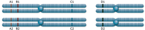
The genotype of the F1 generation resulting from the cross between parent 1 and 2 will be A1A2 B1B2 C1C2 D1D2. Loci A and D are located on different chromosomes and will segregate independently according to the random segregation of chromosomes into gametes. For two different alleles at each locus, four possible combinations can occur, each with a chance of 25%. A and C are unlinked on the same chromosome. They are so far away from each other that recombination occurs between them in 50% of the meioses. The frequencies of all gametes involving alleles at the A and C locus (A1C1, A1C2, A2C1, A2C2) is 0.25, just as it is for the alleles for the A and D loci and the B and D loci. Since locus A and C assort independently, the frequency of double homozygous dominant and double homozygous recessive genotypes (A1A1C1C1, A2A2C2C2) is 0.25×0.25, and the frequency of double heterozygous genotypes (A1A2C1C2) is 0.5 x 0.5.
Loci A and B are linked because they are located in close proximity on the same chromosome resulting in recombination frequencies that are less than 0.5, e.g., 0.1. The difference between the expectation for unlinked loci and the estimated recombination frequency can be used to classify linkage, i.e., the likelihood of two loci being inherited together. To estimate recombination frequencies, non-parental gametes can be counted and divided by the total number of gametes.
Gametic Disequilibrium
Disequilibrium can be created by self-pollination, crossing relatives within a breeding population, mutation, drift, selection, and migration. For example, consider alleles at loci A and D. Let us assume that each contributes to phenotypic variability in flower initiation in an additive manner. Let us also assume selection for earlier flowering (conferred by the A1 and D2 alleles). The impact will be a negative covariance between the alleles at loci A and D, which reduces the genetic variances and creates disequilibrium between those loci. Even though A1 and D2 alleles are physically independent, they become correlated by selection which results in DA1, D2 >0. This is also referred to as the Bulmer effect.
Although individual loci achieve HWE after one generation of random mating, genotype frequencies at two or more loci do not achieve equilibrium jointly after one generation of random mating.
To illustrate this point, consider two populations, one consisting entirely of AABB genotypes and the other consisting entirely of aabb genotypes. Assume they are mixed equally and allowed to mate randomly. The first generation would consist of the three genotypes AABB, AaBb, and aabb in the proportions [latex]\frac{1}{4}:\frac{1}{2}:\frac{1}{4}[/latex]. However, for two loci with two alleles, nine genotypes are possible.
(For n alleles at each locus and k loci, there are [latex](\frac{n(n+1)}{2})^k[/latex] possible genotypes).
Continued random mating would produce the missing genotypes, but they would not appear at the equilibrium frequencies immediately.
Disequilibrium Table
Consider Table 1 below:
| Alleles | A | a | B | b |
| Allele Frequencies | [latex]p_A[/latex] | [latex]1-p_A[/latex] | [latex]p_B[/latex] | [latex]1-p_B[/latex] |
| n/a | n/a | n/a | n/a | n/a |
| Gametic Types | AB | Ab | aB | ab |
| Frequencies at Equilibrium | [latex]p_{AB}[/latex] | [latex]p_A(1-pB)[/latex] | [latex](1-p_A)p_{AB}[/latex] | [latex](1-p_A)(1-p_B)[/latex] |
| Actual Frequencies | R | S | T | U |
| Difference from Equilibrium | [latex]+D_{AB}[/latex] | [latex]-D_{AB}[/latex] | [latex]-D_{AB}[/latex] | [latex]+D_{AB}[/latex] |
A coupling heterozygote would be [latex]\frac {AB}{ab}[/latex] and occur with frequency [latex]\small 2RU[/latex], and the repulsion heterozygote would be [latex]\frac {Ab}{aB}[/latex] occurring with frequency [latex]\small 2ST[/latex]. If the frequency of these two genotypes is equal, the population is in equilibrium, and Equation 1 can be used to estimate the disequilibrium coefficient, D:
[latex]\small D = RU - ST = 0[/latex].
[latex]\textrm{Equation 1}[/latex] Formula for estimating D.
where:
[latex]R, S, T, U[/latex] = the actual gamete frequencies.
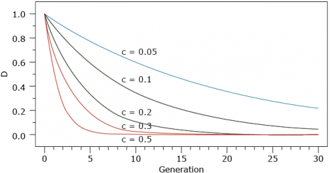
It can be shown that after t generations of random mating, the disequilibrium is given by Equation 2:
[latex]\small D_{t} = D_{0}\left ( 1-c \right )^{t}[/latex].
[latex]\textrm{Equation 2}[/latex] Formula for estimating D after t generations of mating.
where:
[latex]\small D_{0}, D_{t}[/latex] = the disequilibrium in the 0 and t generations, respectively,
[latex]c[/latex] = the recombination frequency, equals[latex]\frac{1}{2}[/latex] for independently segregating loci.
Dissipation of Disequilibrium
The dissipation of disequilibrium relative to generation 0 is given in the figure below:
Deviations from independence at multiple loci are often referred to as linkage disequilibrium, even if linkage is not the cause. Unless two loci are known to reside on the same chromosome the term Gametic Disequilibrium is a less ambiguous term to describe disequilibrium among loci.
Estimation and Testing
Disequilibrium at the A and B loci is a comparison of gametic frequency, [latex]\small p_{AB}[/latex], with the product of allele frequencies, [latex]\small p_Ap_B[/latex]; and is estimated with Equation 3,
[latex]\small \hat{D}_{AB} = \hat{p}_{AB} - \hat{p}_{A}\hat{p}_{B}[/latex]
[latex]\textrm{Equation 3}[/latex] Formula for estimating disequilibrium at two loci.
where:
[latex]\small \hat{D}_{AB}[/latex] = the disequilibrium at loci A and B,
[latex]\textrm {other terms}[/latex] are as defined previously.
The expectation of the estimated disequilibrium between two loci is calculated using Equation 4.
[latex]\small E(\hat{D}_{AB}) = \frac{2n-1}{2n}D_{AB}[/latex].
[latex]\textrm{Equation 4}[/latex] Formula for obtaining the expectation of estimated disequilibrium between two loci.
where:
[latex]\textrm {terms}[/latex] are as defined previously.
The variance of the estimated disequilibrium is calculated using Equation 5.
[latex]\small Var(\hat{D}_{AB}) = {1 \over {2n}}[p_A(1- p_A)p_B(1 -p_B)+(1-2p_A)(1-2p_B)D_{AB}+D^2_{AB}][/latex].
[latex]\textrm{Equation 5}[/latex] Formula for obtaining the variance of estimated disequilibrium between two loci.
where:
[latex]\textrm {terms}[/latex] are as defined previously.
Note the similarities to [latex]\small \hat{D}_{A}[/latex]. Thus, the distribution of estimated disequilibrium between two loci approaches a normal distribution (Equation 6).
[latex]\small \hat{D}_{AB} \; \tilde{N} [E(D_{AB}),\; Var(\hat{D}_{AB})][/latex]
[latex]\textrm{Equation 6}[/latex] Normal distribution equation of [latex]\hat{D}_{AB}[/latex].
where:
[latex]\textrm {terms}[/latex] are as defined previously.
The Z statistic can be obtained using Equation 7;
[latex]Z = \frac{D_{AB}-E(D_{AB})}{\sqrt{Var(D_{AB})}}[/latex].
[latex]\textrm{Equation 7}[/latex] Formula for calculating Z statistic for.
where:
[latex]\textrm {terms}[/latex] are as defined previously.
Chi-Square Statistic
Again, a chi-square statistic for the hypothesis of no disequilibrium can be calculated using Equation 8 and Table 2.
[latex]Z^2 = \chi^2_{AB} = \frac{2nD^2_{AB}}{p_A(1-p_A)p_B(1-p_B)}[/latex].
[latex]\textrm{Equation 8}[/latex] Formula for calculating chi-square statistic,
where:
[latex]\textrm {terms}[/latex] are as defined previously.
| Gamete | AB | AB | AB | AB |
|---|---|---|---|---|
| Observed | [latex]n_AB[/latex] | [latex]n_Ab[/latex] | [latex]n_aB[/latex] | [latex]n_AB[/latex] |
| Expected | [latex]2n\hat p_A\hat p_B[/latex] | [latex]2n\hat p_A \hat p_b[/latex] | [latex]2n\hat p_a \hat p_B[/latex] | [latex]2n\hat p_a \hat p_b[/latex] |
References
Sax, K. 1923. The association of size differences with seed-coat pattern, and pigmentation in Phaseolus vulgaris. Genetics, 8, 552–560.
How to cite this chapter: Beavis, W., A. A. Mahama, & W. Suza. 2023. Linkage. In W. P. Suza, & K. R. Lamkey (Eds.), Quantitative Genetics for Plant Breeding. Iowa State University Digital Press.
