
Chapter 8: Mating Designs
William Beavis; Kendall Lamkey; and Anthony Assibi Mahama
There are many mating designs developed for the purpose of estimating the magnitude of genetic variability in a reference population. This information is most often useful to the plant breeder who is developing a new breeding program in a new crop species or developing a novel germplasm resource for established crop species. For example, large estimates of additive genetic variability and small estimates of genotype by environment variability suggest that rapid progress from selection can be made with minimal allocation of testing resources. While most recently trained plant breeders will assume responsibilities for established plant breeding programs, most established programs begin with an evaluation of genetic variability using one of the many mating designs. Thus, we feel it is instructive to understand the genetic basis upon which these programs were established.
The choice of mating designs is based on:
- The natural mode of reproduction and mating flexibilities of the species.
- The objective(s) in estimating genetic variances such as:
- General interest in knowledge of gene action for quantitative characters
- Making a choice among alternative selection and breeding procedures
- The prediction of response to selection.
- Joint purposes such as estimating genetic variances and simultaneously selecting among progenies or evaluating hybrid combinations
- The precision of the estimates.
Design Setup
Setting up the treatment and experimental designs for mating designs creates unique challenges. Several things need to be considered:
- Ease of making crosses in the species.
- Inbreeding generation of the parents of the crosses.
- The number of parents that will be used (male and female).
- Fixed versus random parents.
- The type of mating design to be used.
- The type of experimental design to be used.
- The environmental design to be used.
Diallel Crosses
Diallel matings (Table 1) are used to make inferences regarding the types of gene effects controlling traits. Diallels are particularly important in cross-pollinated crops and for determining the importance of general combining ability and specific combining ability. Consider the following general mating scheme. This scheme is very similar in structure to the two-way tables we have seen for studying interactions.
| Parents | P1 | P2 | P3 | P4 | Pn | Totals |
|---|---|---|---|---|---|---|
| P1 | Y11 | Y12 | Y13 | Y14 | Y1n | Y1. |
| P2 | Y21 | Y22 | Y23 | Y24 | Y2n | Y2. |
| P3 | Y31 | Y32 | Y33 | Y34 | Y3n | Y3. |
| P3 | Y41 | Y42 | Y43 | Y44 | Y4n | Y4. |
| Pn | Yn1 | Yn2 | Yn3 | Yn4 | Ynn | Yn. |
| Totals | Y.1 | Y.2 | Y.3 | Y.4 | Y.n | Y.. |
Number of Diallel Crosses and Entries
Let us consider the number of diallel crosses for n parents with and without reciprocal crosses. The number of entries is the number that would have to be evaluated if the parents were included in the experiment (Table 2).
| Without Reciprocals | With Reciprocals | |||
| No. of Parents | No. of Crosses | Number of Entries | No. of Crosses Including Reciprocals | Number of Entries |
| [latex]n[/latex] | [latex]\frac{n(n-1)}{2}[/latex] | [latex]\frac{n(n-1)}{2}[/latex] | [latex]n(n-1)[/latex] | [latex]n(n-1)[/latex] |
| 5 | 10 | 15 | 20 | 20 |
| 6 | 15 | 21 | 30 | 30 |
| 7 | 21 | 28 | 42 | 42 |
| 8 | 28 | 36 | 56 | 56 |
| 9 | 36 | 45 | 72 | 72 |
| 10 | 45 | 55 | 90 | 90 |
| 11 | 55 | 66 | 110 | 110 |
| 12 | 66 | 78 | 132 | 132 |
| 13 | 78 | 91 | 156 | 156 |
| 14 | 91 | 105 | 182 | 182 |
| 15 | 105 | 120 | 210 | 210 |
| 20 | 190 | 210 | 380 | 380 |
| 50 | 1225 | 1275 | 2450 | 2450 |
| 100 | 4950 | 5050 | 9900 | 9900 |
Types of Diallel Analysis
| Model | Method | Parents Included | Crosses | Reciprocals |
|---|---|---|---|---|
| I (Fixed) | 1 | Yes | Yes | Yes |
| I (Fixed) | 2 | Yes | Yes | No |
| I (Fixed) | 3 | No | Yes | Yes |
| I (Fixed) | 4 | No | Yes | No |
| II (Random) | 1 | Yes | Yes | Yes |
| II (Random) | 2 | Yes | Yes | No |
| II (Random) | 3 | No | Yes | Yes |
| II (Random) | 4 | No | Yes | No |
Common Diallel Experiment
The most common diallel experiment is conducted with selected parents, which means a fixed effects analysis where only gene effects and not variance will be estimated (Table 3). The reason for this is simple: It is very hard to sample a population adequately with a diallel. Diallels are useful mating designs, however, despite this limitation.
Therefore, we will not present any analyses related to estimating variance components — only gene effects. This makes this section somewhat out of place, but it fits in with the other mating designs from the structural point of view. The analyses we will present are a combination of those presented by Griffing (1956) and Gardner and Eberhart (1966).
Methods 2 and 4 are the most common types of diallels. Most scientists grow the parents and the crosses or just the crosses. The method 4 analysis is, however, the most commonly used analysis because Griffing assigns specific combining ability effects to the parents per se, and these are hard to interpret relative to Sprague and Tatum’s (1942) definitions of general and specific combining ability.
The general model underlying the diallel can be written as in Equation 1:
[latex]Y_{ijk} = \mu + g_{i}+ g_{j} + s_{ij} + r_k + e_{ijk},[/latex]
[latex]\textrm{Equation 1}[/latex] General linear model for diallel design experiments.
where:
[latex]\mu[/latex] = the mean,
[latex]g_{i}[/latex] = the general combining ability effect (marginal effect) of the ith parent,
[latex]g_{j}[/latex] = the general combining ability effect (marginal effect) of the jth parent,
[latex]s_{ij}[/latex] = the specific combining ability effect (interaction effect) of the ith and jth parents,
[latex]r_{k}[/latex] = the effect of the kth replication,
[latex]e_{ijk}[/latex] = the residual (or error).
An ANOVA Table for Diallels is shown in Table 4.
| Source | df | df (n = 10) |
SS | MS | EMS (Model I – Fixed Effects) |
|---|---|---|---|---|---|
| Replications | [latex]r-1[/latex] | [latex]r-1[/latex] | n/a | n/a | n/a |
| Entries | [latex]\frac{n(n-1)}{2}-1[/latex] | 44 | [latex]S2[/latex] | [latex]M2[/latex] | [latex]\sigma_{\varepsilon}^{2} + r \delta_{t}^{2}[/latex] |
| Among Margins | [latex]n-1[/latex] | 9 | [latex]S21[/latex] | [latex]M21[/latex] | [latex]\sigma_{\varepsilon}^{2} + (\frac{n-2}{n-1})\sum_i g_{i}^{2}[/latex] |
| Among cells/Margins | [latex]\frac{n(n-3)}{2}[/latex] | 35 | [latex]S22[/latex] | [latex]M22[/latex] | [latex]\sigma_{\varepsilon}^{2} + (\frac{2r}{n(n-3)})\sum_{i\prec j} s_{ij}^{2}[/latex] |
| Error | [latex](r-1)(\frac{n(n-1)}{2}-1)[/latex] | 44[latex]r-1[/latex] | [latex]S1[/latex] | [latex]M1[/latex] | [latex]\sigma_{\varepsilon}^{2}[/latex] |
F-Tests
Model I F-Tests: For among cells/margins and among margins are, respectively,
[latex]F = \frac{M_{22}}{M_1} \text{, and } [/latex]
[latex]F = \frac{M_{21}}{M_1}[/latex]
These F-tests evaluate whether differences among the parents and crosses within parents are significant. Also, it is possible to show that the effects can be estimated using Equation 2:
[latex]\hat u = \frac{2}{n(n-1)}Y..[/latex],
[latex]\hat g_i = \frac{1}{n(n-2)}(nY_{i.} - 2Y..)[/latex],
[latex]\hat s_{ij} = Y_{ij}- \frac{1}{n-2}(Y_{i.} Y_{.j}) \frac{2}{(n-1)(n-2)}Y..[/latex],
[latex]\textrm{Equation 2}[/latex] Formulae for estimating mean, gca, and sca effects.
where:
[latex]\hat u[/latex] = estimated mean,
[latex]n[/latex] = number of parents,
[latex]\hat g_i[/latex] = estimate of gca effect of genotype i,
[latex]\hat s_{ij}[/latex] = estimate of sca effect of genotypes i and j,
[latex]Y_{..}[/latex] = grand total,
[latex]Y_{i.}[/latex] = sum of parent i across all parents,
[latex]Y_{.j}[/latex] = sum of parent j across all parents,
[latex]Y_{ij}[/latex] = phenotype of cross ij .
The variances of the effects can be estimated with Equation 3:
[latex]V(\hat u)= \frac{2}{n(n-1)}\hat\sigma_{\bar{Y}}^{2}[/latex]
[latex]V(\hat g_i) = \frac{1}{n(n-2)}\hat\sigma_{\bar{Y}}^{2}[/latex]
[latex]V(\hat s _{ij})= \frac{n-3}{n-1}\hat \sigma _{\bar{Y}}^{2}, (i\neq j)[/latex]
[latex]\text{and}[/latex]
[latex]\hat \sigma_{\bar{Y}}^{2} = \frac{\hat \sigma_{\varepsilon}^{2}}{r}= \frac{M_1}{r}[/latex]
[latex]\textrm{Equation 3}[/latex] Formulae for estimating variances of estimated of mean, gca, sca effects and error,
where:
[latex]\hat \sigma_{\bar{Y}}^{2}[/latex] = estimates variance of average phenotype,
other terms are as defined previously.
Gardner and Eberhart Diallel Analysis II
The Gardner and Eberhart Analysis II for the diallel is a more general analysis designed for the case of when the diallel includes random mating varieties. The model is best laid out by starting with the following single locus theory for the [latex]j^{th}[/latex] variety and [latex]i^{th}[/latex] locus (Table 5):
| Frequency | Genotype | Genotypic value |
|---|---|---|
| [latex]p^2_{ji}[/latex] | AA | [latex]\mu' a_i[/latex] |
| [latex]2p_{ji}(1-p_{ji})[/latex] | Aa | [latex]\mu' \delta_i[/latex] |
| [latex](1-p_{ji})^2[/latex] | aa | [latex]\mu' - a_i[/latex] |
Where, [latex]\mu' = \frac{AAaa}{2}[/latex].
The population mean can be written as in Equation 4:
[latex]\mu' \sum_i(2p_{ji}-1) \alpha_{i} + 2\sum_i(p_{ji}-p_{ji}^{2})\delta_i[/latex]
[latex]\textrm{Equation 4}[/latex] Formula for calculating the population mean,
where:
[latex]p, 1-p[/latex] = frequencies of the two allele.
[latex]\mu'[/latex] = average genotypic value,
[latex]\alpha _i, \delta_i[/latex] = coded genotypic values.
Equations
Let [latex]a'_j=\sum_i(2p_{ji} - 1)\alpha_i; \quad \bar a = \frac{1}{n}\sum_j a'_j; \quad a_j=a'_j-\bar a; and\quad \mu = \mu'+ \bar a[/latex].
Similarly, let [latex]d_j = 2\sum_i({p}_{\small{ji}}-{p}_{\small{ji}}^{2})\delta_i; \quad h_{jj'}=\sum_i({p}_{\small{ji}}-{p}_{\small{ji}}^{2})^2\delta_i[/latex].
Then, the population mean can be written as in Equation 5:
[latex]\textrm{pop mean}=\mu' + a'_j + d_j =\mu + a_j + d_j[/latex]
[latex]\textrm{Equation 5}[/latex] Formula for the population mean.
where:
[latex]\mu[/latex] = the mean,
[latex]\mu'[/latex] = average genotypic value of AA & aa,
[latex]a[/latex] =genotypic value of AA, aa genotypes,
[latex]d[/latex] = genotypic value of Aa genotype.
A population cross mean can be written as in Equation 6:
[latex]C_{jj'}= \mu + \frac{1}{2}(a_j a_{j'}) + \frac{1}{2}(d_j + d_{j'} + h_{jj'})[/latex].
[latex]\textrm{Equation 6}[/latex] Formula for the population cross mean.
where:
[latex]C_{jj'}[/latex] = mean of the “variety cross” from two parents,
[latex]\mu[/latex] = the mean of all crosses,
[latex]a[/latex] = the additive effect,
[latex]d[/latex] = the dominance effect,
[latex]h_{jj'}[/latex] = the heterosis effect.
If the varieties, varieties selfed, population crosses, population crosses selfed, and population crosses random mated are included in the analysis, then all of these genetic effects can be estimated. Usually, this is not the case, and only varieties and variety crosses are included in the analysis, which are confounded, and they have to be estimated together. We can then define the following parameters:
The mean of all parental varieties included in the analysis is written as in Equation 7:
[latex]\mu_v=\mu \frac{1}{n}\sum_{j} d_j; \quad =\mu + \bar d[/latex]
[latex]\textrm{Equation 7}[/latex] Formula for mean when all parental varieties are included.
where:
[latex]\mu_v[/latex] = the mean of all parental varieties included in the analysis,
[latex]\mu[/latex] = the mean,
[latex]d[/latex] = dominance effect,
[latex]\bar d[/latex] = average dominance effects.
The variety effect when parents are included in the analysis is written as in Equation 8:
[latex]v_j = a_j + (d_j + \bar d)[/latex]
[latex]\textrm{Equation 8}[/latex] Formula for estimating variety effects with parents included.
where:
[latex]v[/latex] = the variety effect when parents are included,
[latex]a, d[/latex] are as defined previously.
Models
We can then fit the following four models to the data (Equation 9):
[latex]\eqalign {Y_{jj'} &=\mu_v + \frac{1}{2}(v_j v_{j'}) \\ Y_{jj'} &=\mu_v + \frac{1}{2}(v_j v_{j'}) + γ\bar h \\ Y_{jj'} &=\mu_v + \frac{1}{2}(v_j v_{j'}) + γ\bar h + γ(h_j h_i') \\ Y_{jj'} &=\mu_v + \frac{1}{2}(v_j v_{j'}) + γ\bar h + γ(h_j h_{j'}) + γs_{jj'}}[/latex]
[latex]\textrm{Equation 9}[/latex] Linear models for estimating different genetic effects on phenotype,
where:
[latex]y=\begin{Bmatrix} 0\ when\ j=j'\\ 1\ when\ j\neq j' \end{Bmatrix}[/latex],
[latex]Y_{jj'}[/latex] = phenotype of j by j’ progeny.
ANOVA Table
The following ANOVA table can be written as in Table 6:
| Source | df | Sum of squares |
| Populations | [latex][n(n-1)/2]-1[/latex] | [latex]S'[/latex] |
| Varieties [latex](v_j)[/latex] | [latex]n-1[/latex] | [latex]S'_1=(B'G)_1-CF[/latex] |
| Heterosis[latex](h_{jj'})[/latex] | [latex]n(n - 1)/2[/latex] | [latex]S'_1 = (B'G)_1-(B'G)[/latex] |
| Average [latex](\bar h)[/latex] | [latex]1[/latex] | [latex]S'_{21} = (B'G)_2-(B'G)_1[/latex] |
| Variety [latex](h_j)[/latex] | [latex]n-1[/latex] | [latex]S'_{22} = (B'G)_3-(B'G)_2[/latex] |
| Specific [latex](s_{jj'})[/latex] | [latex]\frac {n(n-3)}{2}[/latex] | [latex]S'_{23} = (B'G)_4-(B'G)_3[/latex] |
Equivalent Analysis
An equivalent analysis can be made with just the crosses as follows:
The mean of crosses in the diallel can be estimated as follows:
[latex]\eqalign {Let: \;\mu_c &= \mu_v \bar h &= \mu \bar d \bar h}[/latex];
The variety effect in crosses = general combining ability effect = [latex]g_j=\frac{1}{2}v_j h_j[/latex], then the mean of crosses is written as in Equation 10:
[latex]C_{jj'} = \mu_c + g_j + g_j' + s_{jj'}[/latex]
[latex]\textrm{Equation 10}[/latex] Model for analysis with only crosses included.
where:
[latex]s_{jj'}[/latex] = specific heterosis from variety j by variety j’ mating,
[latex]\sum_jg_j=0[/latex],
[latex]\sum_{j\neq j'}s_{jj'} = 0[/latex].
Analysis III of Gardner and Eberhart
The following ANOVA (Table 7) can be written (Analysis III of Gardner and Eberhart)
| Source | Degrees of Freedom | Sum of squares |
| Population | [latex][n(n-1)/2]-1[/latex] | n/a |
| Varieties ([latex]v_j[/latex]) | [latex]n-1[/latex] | [latex]S''_1[/latex] |
| Varieties vs. crosses ([latex]\bar{h}[/latex]) | [latex]1[/latex] | [latex]S''_2[/latex] |
| Crosses([latex]x_{jj'}[/latex]) | [latex][n(n-1)/2]-1[/latex] | [latex]S''_3[/latex] |
| GCA ([latex]g_{j}[/latex]) | [latex]n-1[/latex] | [latex]S''_{31}[/latex] |
| SCA ([latex]s_{jj'}[/latex]) | [latex]\frac {n(n-3)}{2}[/latex] | [latex]S''_{32}[/latex] |
The analysis of Crosses, GCA, and SCA is all that can be done if only the crosses are included in the analysis. This analysis is equivalent to the Model 4 analysis of Griffing. If varieties or parents are also included, then the analysis, Varieties, and Varieties vs. Crosses can also be calculated.
Analysis III is related to Analysis II in the following ways that the (sjj’) are the same in the two analyses S’21 = S”2, meaning that average heterosis is simply a contrast of the mean of the varieties with the mean of the crosses (Equation 11).
[latex]S''_{1} + S''_{31} = S'_{1} + S'_{22}, \textrm{since}\ g_j= \frac{1}{2}v_j h_j[/latex]
[latex]\textrm{Equation 11}[/latex] Formula for calculating average heterosis.
where:
[latex]S''_{1}[/latex] = effects of variety 1,
[latex]S''_{2}[/latex] = effects of variety 2,
[latex]S''_{3}[/latex] = effects of crosses,
[latex]S''_{31}[/latex] = GCA effects,
[latex]S''_{32}[/latex] = SCA effects.
North Carolina Design I

- Consider m male plants:
- each of which is mated to f female plants,
- to produce n full-sib families within each male,
- for a total of mf half-sib families.
- There is a total of m half-sib families.
- Different female plants are used to cross with each male.
- The progeny P are grown in a replicated experiment design.
The model for analysis is written as in Equation 12:
[latex]Y_{ijk}=\mu + m_{i} + f_{ij} + r_{k} + e_{ijk}[/latex]
[latex]\textrm{Equation 12}[/latex] General linear model for NC I experiments.
where:
[latex]\mu[/latex] = the mean,
[latex]m_{i}[/latex] = the effect of male i,
[latex]f_{ij}[/latex] = the effect of female j when crossed to male i,
[latex]r_{k}[/latex] = replication effect,
[latex]e_{ijk}[/latex] = the residual.
ANOVA Table
Then the ANOVA (Table 8) can be written as:
| Source of Variation | d.f. | MS | EMS |
|---|---|---|---|
| Replications | [latex]r-1[/latex] | n/a | n/a |
| Males | [latex]m-1[/latex] | M4 | [latex]\sigma + r\sigma^2_{f(m)} + rf\sigma^2_m[/latex] |
| Females/Males | [latex]m(f-1)[/latex] | M3 | [latex]\sigma^2 + r\sigma^2_{f(m)}[/latex] |
| Error | [latex](mf-1)(r-1)[/latex] | M2 | [latex]\sigma^2[/latex] |
| Total | [latex]rmf-1[/latex] | n/a | n/a |
| Within | [latex]rmf(k-1)[/latex] | M1 | [latex]\sigma^2_W[/latex] |
The table can be rewritten in terms of the covariance of relatives as follows (Table 9):
| Source of Variation | d.f. | MS | EMS |
|---|---|---|---|
| Replications | [latex]r-1[/latex] | n/a | n/a |
| Males | [latex]m-1[/latex] | M4 | [latex]\sigma^2 + r[Cov(FS) - Cov(HS)] + rfCov(HS)[/latex] |
| Females/Males | [latex]m(f-1)[/latex] | M3 | [latex]\sigma^2 + r[Cov(FS) - Cov(HS)][/latex] |
| Error | [latex](mf-1)(r-1)[/latex] | M2 | [latex]\sigma^2[/latex] |
| Total | [latex]rmf-1[/latex] | n/a | n/a |
| Within | [latex]rmf(k-1)[/latex] | M1 | [latex]\sigma^2_W[/latex] |
[latex]And \quad \sigma^2_u= \frac {\sigma^2_{\mu \varepsilon} [\sigma^2_G - Cov(FS)]}{k}[/latex]
Variance Estimates
Estimation of variance of the various components is as in Equation 13:
[latex]\hat{\sigma}^2_m=Cov(HS)=\frac{M_4-M_3}{rf}; \quad \hat{\sigma}^2_{f(m)}= Cov(FS)-Cov(HS)=\frac{M_4-M_3}{rf}[/latex]
[latex]\textrm{Equation 13}[/latex] Formulae for calculating variance components for NC I.
where:
[latex]\hat{\sigma}^2_m[/latex] = variance of males,
[latex]\hat{\sigma}^2_{f(m)}[/latex] = variance of males within females,
[latex]Cov(HS)[/latex] = covariance of half-sibs,
[latex]Cov(FS)[/latex] = covariance of full-sibs.
So, ignoring epistasis, the variances are written as in Equation 14:
[latex]\hat{\sigma}^2_m=\frac{(1-F_m)}{4}\sigma^2_A; \quad \hat{\sigma}^2_{f(m)}=\frac{(2 + F_m + F_f)}{4}\sigma^2_A + \frac{(1 + F_m)(1 + F + f)}{4}\sigma^2_D-\bigg[\frac{(1 +F_m)}{4}\sigma^2_A\bigg][/latex].
[latex]\textrm{Equation 14}[/latex] Alternative formulae for calculating variance components.
where:
[latex]\sigma^2_A[/latex] = the additive variance,
[latex]\sigma^2_D[/latex] = the dominance variance,
[latex]F_m[/latex] = the inbreeding coefficient of the male parent,
[latex]\hat{\sigma}^2_{f(m)}[/latex] = estimated variance of male within females,
[latex]F_f[/latex] = the inbreeding coefficient of the female parent,
[latex]f[/latex] = effects of females.
Consider the case when all the parents are noninbred, i.e., Fm = Ff = 0. The variances are written as in Equation 15:
[latex]\eqalign { \hat\sigma^2_m &= \frac{1}{4}\sigma^2_A; \quad \hat \sigma^2_{f(m)}&= \frac{1}{2}\sigma^2_A + \frac{1}{4}\sigma^2_D-[\frac{1}{4}\sigma^2_A]=\frac{1}{4}(\sigma^2_A +\sigma^2_D); \quad \hat\sigma ^2_A &= 4\hat \sigma ^2_m; \quad \hat\sigma^2_D &=4(\hat\sigma^2_{f(m)}-\sigma^2_m) }[/latex]
[latex]\textrm{Equation 15}[/latex] Formulae for calculating variance component when all the parents are noninbred.
where:
[latex]terms[/latex] are as defined previously.
When both the male and female parents are inbred, i.e., Fm = Ff = 1, then the variances can be estimated as written in Equation 16:
[latex]\eqalign { \hat \sigma^2_m &=\frac{1}{2}\sigma^2_A; \quad \hat\sigma^2_{f(m)} &= \sigma^2_A + \sigma^2_D-[\frac{1}{2}\sigma^2_A]=\sigma^2_A + \frac{1}{2}\sigma^2_D; \quad \hat\sigma^2_A &= 2\sigma^2_m; \quad \hat\sigma^2_D &=(\hat\sigma^2_{f(m)}-2\hat\sigma^2_m) }[/latex]
[latex]\textrm{Equation 16}[/latex] Formulae for calculating variance component when all the parents are inbred.
where:
[latex]terms[/latex] are as defined previously.
North Carolina Design II
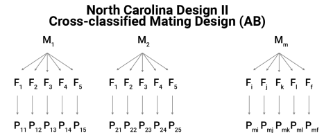
- Consider m male plants,
- each of which is mated to f female plants,
- to produce f full-sib families within each male,
- for a total of mf half-sib families.
- There is a total of m f half-sib families.
- The same female plants are crossed with each male.
- The progeny P are grown in a replicated experiment design.
The design is related to the diallel and another simpler way to represent the design is (Table 10):
| Parents | M1 | M2 | M3 | M4 | Totals |
|---|---|---|---|---|---|
| F5 | Y15 | Y25 | Y35 | Y45 | Y.5 |
| F6 | Y16 | Y26 | Y36 | Y46 | Y.6 |
| F7 | Y17 | Y27 | Y37 | Y47 | Y.7 |
| F8 | Y18 | Y28 | Y38 | Y48 | Y.8 |
| Totals | Y1. | Y2. | Y3. | Y4. | Y.. |
Model
The model for analysis is written as in Equation 17:
[latex]Y_{ijk} = µ + m_{i} + f_{ij} + mf_{ij} + r_{k} + e_{ijk}[/latex]
[latex]\textrm{Equation 17}[/latex] Formulae for calculating variance components for NC II.
where:
[latex]\mu[/latex] = mean,
[latex]m_{i}[/latex] =the effect of male i,
[latex]f_{j}[/latex] = the effect of female j,
[latex]mf_{ij}[/latex] = the interaction effect of female j when crossed to male i,
[latex]r_k[/latex] = replication effect,
[latex]e_{ijk}[/latex] =the residual.
ANOVA Table
The ANOVA is shown in Table 11.
| Source of Variation | d.f. | MS | EMS |
|---|---|---|---|
| Replications | [latex]r-1[/latex] | n/a | n/a |
| Males (M) | [latex]m-1[/latex] | M5 | [latex]\sigma^2 + r\sigma^2_{mf} + r\sigma^2_{m}[/latex] |
| Females (F) | [latex]f-1[/latex] | M4 | [latex]\sigma^2 + r\sigma^2_{mf} + rm\sigma_{f}^2[/latex] |
| M x F | [latex](m - 1)(f - 1)[/latex] | M3 | [latex]\sigma^2 + r\sigma^2_{mf}[/latex] |
| Error | [latex](mf - 1)(r - 1)[/latex] | M2 | [latex]\sigma^2[/latex] |
| Total | [latex]rmf - 1[/latex] | n/a | n/a |
| Within | [latex]rmf (k - 1)[/latex] | M1 | [latex]\sigma^2_w[/latex] |
Covariance of Relatives
The table can be rewritten in terms of the covariance of relatives as follows (Table 12):
| Source of Variation | d.f. | MS | EMS |
|---|---|---|---|
| Replications | [latex]r-1[/latex] | n/a | n/a |
| Males (M) | [latex]m-1[/latex] | M5 | [latex]\sigma^2 + r[Cov(FS) - Cov(HS_m) - Cov(HS_f)] + rfCov(HS_m)[/latex] |
| Females (F) | [latex]f-1[/latex] | M4 | [latex]\sigma^2 + r[Cov(FS) - Cov(HS_m) - Cov(HS_f)] + rmCov(HS_f)[/latex] |
| M x F | [latex](m - 1)(f - 1)[/latex] | M3 | [latex]\sigma^2 + r[Cov(FS) - Cov(HS_m) - Cov(HS_f)][/latex] |
| Error | [latex](mf - 1)(r - 1)[/latex] | M2 | [latex]\sigma^2[/latex] |
| Total | [latex]rmf - 1[/latex] | n/a | n/a |
| Within | [latex]rmf (k - 1)[/latex] | M1 | [latex]\sigma^2_w[/latex] |
[latex]\text{And } \quad\sigma^2_u = \frac{\sigma^2_{u\varepsilon} [\sigma^2_G - Cov(FS)]}{k}[/latex]
Estimation
Variance components are estimated as written in Equation 18:
[latex]\hat\sigma^2_m=Cov(HS_m)=\frac{M5-M3}{rf}; \quad \hat\sigma^2 = Cov(HS_f)=\frac{M4-M3}{rm}; \quad \hat\sigma^2_{mf}= \big[Cov(FS)-Cov(HS_m)-Cov(HS_f)\big]=\frac{M3-M2}{r}[/latex]
[latex]\textrm{Equation 18}[/latex] Formula for estimating covariance of relatives,
where:
[latex]\hat\sigma^2_m[/latex] = estimated variance of males,
[latex]\hat\sigma^2_f[/latex] = estimated variance of females,
[latex]\hat\sigma^2_{mf}[/latex] = estimated variance of male by female cross (full-sibs),
[latex]Cov(FS)[/latex] = covariance of full-sibs,
[latex]Cov(HS_m)[/latex] = covariance of half-sibs with common male,
[latex]Cov(HS_f)[/latex] = covariance of half-sibs with common female.
Variance Estimates
Ignoring epistasis, variance components are estimated as written in Equation 19.
[latex]\eqalign {\hat\sigma^2m &=\frac{(1+ F_m)}{4}\sigma^2_A; \quad \hat\sigma^2_f &=\frac{(1 + F_f)}{4}\sigma^2_A; \quad \hat\sigma^2_{mf} &=\frac{(2 + F_m + F_f)}{4}\sigma^2_A + \frac{(1 + F_m)(1 + F_f)}{4}\sigma^2_D-\bigg[\frac{(1-F_m)}{4} + \frac{1 + F_f)}{4}\bigg]\sigma^2_A }[/latex]
[latex]\textrm{Equation 19}[/latex] Formula for calculating variance estimates, ignoring epistasis.
where:
[latex]terms[/latex] are as defined previously.
Consider the case when all the parents are noninbred, i.e., Fm = Ff = 0. Variance components are estimated as written in Equation 20:
[latex]\hat\sigma^2_m=\frac{1}{4}\sigma^2_A; \quad \hat\sigma^2_f=\frac{1}{4}\sigma^2_A; \quad \require{cancel}\hat\sigma^2_{mf}={\cancel{\color{#555}{\frac{1}{2}\sigma^2_A}}} + \frac{1}{4}\sigma^2_D-{\cancel{\color{#555}{[\frac{1}{4} +\frac{1}{4}]\sigma^2_A}}}=\frac{1}{4}\sigma^2_D; \quad \hat\sigma^2_A=4(\frac{\hat\sigma^2_m +\hat\sigma^2_f}{2})=2(\hat\sigma^2_m + \hat\sigma^2_f); \quad\sigma^2_D=4\hat\sigma^2_{mf}[/latex]
[latex]\textrm{Equation 20}[/latex] Formulae for estimating variance components when male and female parents are noninbred,
where:
[latex]terms[/latex] are as defined previously.
When both the male and female parents are inbred, i.e., Fm = Ff = 1, then variance components are estimated as written in Equation 21:
[latex]\hat\sigma^2_{m}=\tfrac{1}{2}\sigma _{A}^{2}; \quad \hat\sigma^2_f=\tfrac{1}{2}\sigma^2_A ; \quad\hat\sigma^2_{mf}={\sigma^2_A} + \sigma^2_D-[\tfrac{1}{2} + \tfrac{1}{2}]\sigma^2_A = \sigma^2_D ; \quad\sigma^2_A=\hat\sigma^2_m +\hat\sigma^2_f; \quad \sigma^2_m=\hat\sigma^2_{mf}[/latex]
[latex]\textrm{Equation 21}[/latex] Formulae for estimating variance components when male and female parents are inbred,
where:
[latex]terms[/latex] are as defined previously.
North Carolina Design III
The main use of Design III is for estimating the average degree of dominance.
North Carolina Design III Backcross Design is shown in Fig. 3.

This design involves crossing two inbred lines and obtaining the F1 and F2 generations. An individual F2 plant is then backcrossed to each of the inbred parents generating a pair of progeny using the F2 plants and pollen parents. Then for n F2 plants, there are 2n progenies produced, and the model is as written in Equation 22:
[latex]Y_{ijk} = µ + l_{i} + m_{j} + ml_{ij} + r_k + e_{ijk}[/latex]
[latex]\textrm{Equation 22}[/latex] Linear model for estimating average degree of dominance.
where:
[latex]\mu[/latex] = the mean,
[latex]l_{i}[/latex] = contrast of the inbred parents i = 1, 2
[latex]m_{j}[/latex] = the effect of F2 parent j,
[latex]ml_{ij}[/latex] = the interaction effect of inbred parent i and F2 plant i,
[latex]r_k[/latex] = replication effect,
[latex]e_{ijk}[/latex] =the residual.
ANOVA Table
An ANOVA Table for North Carolina Design III is shown in Table 13.
| Source of Variation | d.f. | MS | EMS |
|---|---|---|---|
| Replications | [latex]r - 1[/latex] | n/a | n/a |
| Inbred Lines | [latex]1[/latex] | n/a | n/a |
| F2 parents | [latex]n - 1[/latex] | M3 | [latex]\sigma^2 + 2r\sigma^2_m[/latex] |
| F2 parent x inbred line | [latex]n - 1[/latex] | M2 | [latex]\sigma^2 + r\sigma^2_{ml}[/latex] |
| Error | [latex](2n - 1)(n - 1)[/latex] | M1 | [latex]\sigma^2[/latex] |
| Total | [latex]rmf - 1[/latex] | n/a | n/a |
Estimation
Variance components are estimated as written in Equation 23:
[latex]\hat\sigma^2_m=\frac{M3-M1}{2r}=\frac{1}{8}\sum_ia^2_i, \quad \hat\sigma^2_{ml} = \frac{M2-M1}{r}=\frac{1}{4}\sum_1d^2_i[/latex]
[latex]\textrm{Equation 23}[/latex] Formulae for estimating effects of parents and the interaction effect of inbred parents and F2 plants,
where:
[latex]\sum[/latex] = the summation is over i loci,
[latex]\hat\sigma^2_m[/latex] = estimated variance of F2 parents i = 1, 2
[latex]\hat\sigma^2_{ml}[/latex] = estimated variance of the interaction effect of the parent and F2 plant.
F-Tests
Remember that in an F2 population, additive and dominance variances are written as in Equation 24
[latex]\sigma^2_A=\frac{1}{2}\sum_ia^2_i, and \quad \sigma^2_D=\frac{1}{4}\sum_id^2_i[/latex]
[latex]\textrm{Equation 24}[/latex] Formula for total genetic variance for and F3 population,
so that variance components are estimated as written in Equation 25,
[latex]\hat\sigma^2_m=\frac{1}{4}\sigma^2_A, and \quad \hat\sigma^2_{ml}=\sigma^2_D[/latex]
[latex]\textrm{Equation 25}[/latex] Formula for total genetic variance for and F3 population.
where:
[latex]\hat\sigma^2_m; \hat\sigma^2_{ml}[/latex] are as defined previously,
[latex]\sigma^2_A[/latex] = additive variance,
[latex]\sigma^2_D[/latex] = dominance variance.
Note that this design is very specialized for the specific case of F2 populations when p = q = 0.5. This design provides exact F-tests of two important hypotheses:
- The null hypothesis of no dominance. This is tested by: F=M2/M1, and if this F-test is significant, then it means that [latex]d \succ |0|[/latex] and there is no dominance.
- The null hypothesis is that dominance is complete. If there is complete dominance, then the ratio, M3/M2=1.
A significant departure of this ratio from one indicates that [latex]d[/latex] departs significantly from 1.
References
Gardner, C. O, and A. S., Eberhart. 1966. Analysis and interpretation of the variety cross diallel and related populations. Biometrics, 22(3):439-52.
Griffing, B. 1956. Concept of General and Specific Combining Ability in Relation to Diallel Crossing Systems. Aust. J. Biol. Sci. 9: 463-93.
Sprague, G. F., and Tatum, L. A. 1942. General Vs Specific Combining Ability in Single Crosses of Corn. J. Amer. Soc. Agron. 34: 923-32.
How to cite this chapter: Beavis, W., K. Lamkey, and A. A. Mahama. 2023. Mating Designs. In W. P. Suza, & K. R. Lamkey (Eds.), Quantitative Genetics for Plant Breeding. Iowa State University Digital Press.
