
Chapter 3: Resemblance Between Relatives
William Beavis; Kendall Lamkey; and Anthony Assibi Mahama
Plant breeding populations, by definition, employ methods that force populations into states of disequilibrium. Plant breeders do not mate infinite (or even large) numbers of parents; thus, drift has a major impact on population disequilibrium. They select the parents that will be used in mating; thus, selection linkage and pleiotropy affect the population structure. New lines from external breeding projects are often introduced to the breeding nurseries, thus migration affects the structure of plant breeding populations. After the passage of the Plant Variety Protection Act, plant breeders working in the commercial sector began to keep breeding records for purposes of protecting intellectual property. An unintended consequence has been the application of mixed linear models to produce predictors of performance, originally developed by animal breeders. These methods are predicated on the use of coefficients of relationship among cultivars with known performance and progeny with unknown or limited information on performance.
- Utilize population genetic concepts as a foundation to understand coefficients of inbreeding, parentage, and relationship.
- Calculate coefficients of parentage and inbreeding.
Background
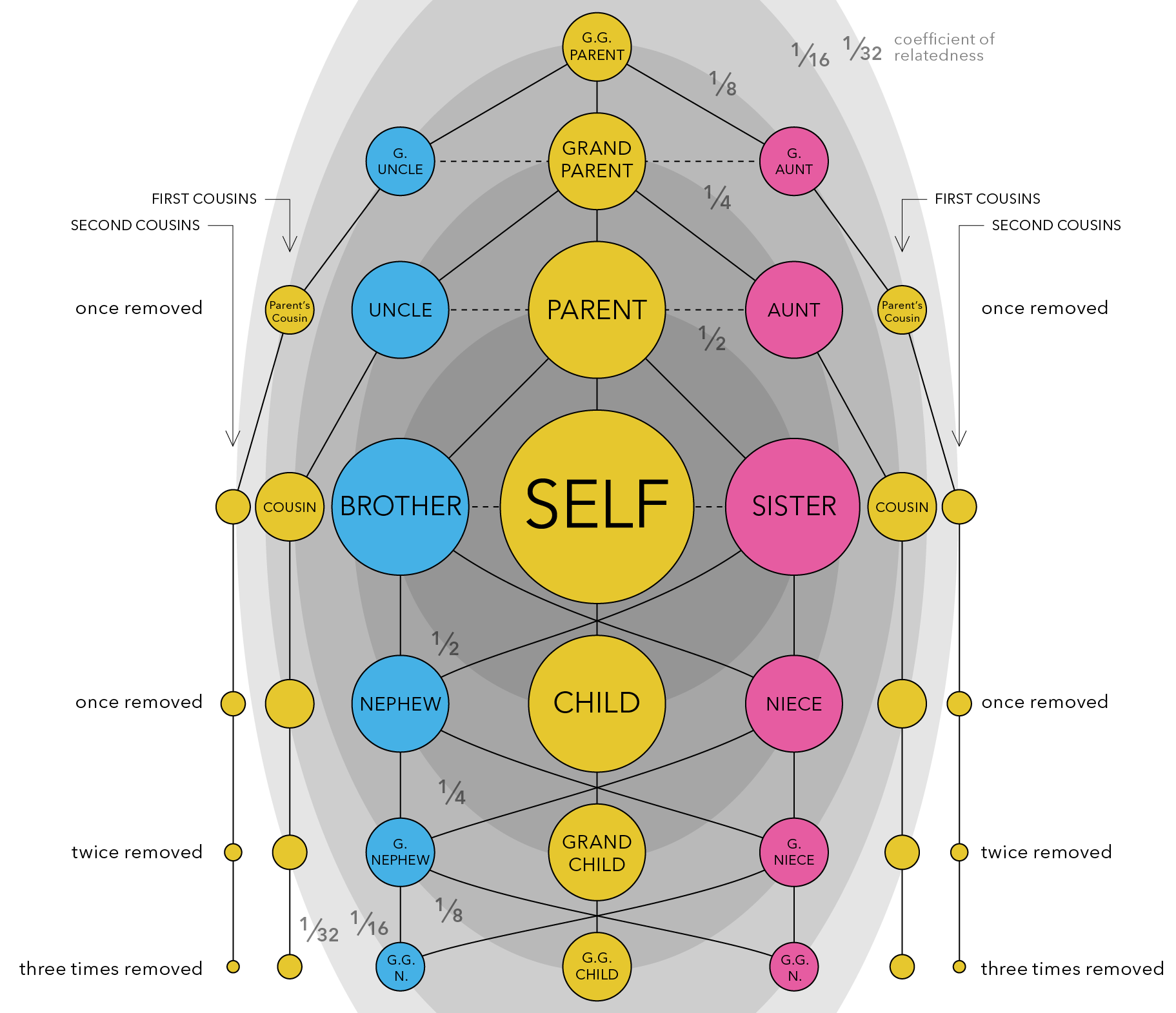
The calculation of coefficients of relationships and inbreeding were originally developed as path coefficients by Sewall Wright and identity by descent by Gustave Malécot. The calculations were simplified by Emik and Terrill (1949) and extended to all possible measures of identity by Cockerham (1971). Example relatedness in humans is shown in Fig. 2.
Herein we introduce inbreeding and parentage as deviations (disequilibrium) from Hardy Weinberg Equilibrium. In other words, the calculations of all of these measures are based on a reference population and the reference population must be defined or else the calculated values have no meaning.
Coefficient of Inbreeding
Let us consider a random mating diploid population consisting of [latex]N[/latex] individuals: Because there are [latex]2N[/latex] gametes, the probability that two mating gametes are identical by descent is [latex]1\over{2N}[/latex]. Therefore, [latex]F_1 = {{1}\over{2N}}[/latex]. The remaining proportion of zygotes [latex]1 - {1\over{2N}}[/latex] carry genes that are independent in origin from generation 1. Therefore, the probability of identical homozygotes in generation 2 is represented by Equation 1:
[latex]F_2 = {1\over{2N}} + (1 - {1\over{2N}})F_1[/latex],
[latex]\textrm{Equation 1}[/latex] Formula for calculating the probability of identical homozygotes in generation 2.
where:
[latex]F_{1}, F_{2}[/latex] = the inbreeding coefficients of generations 1 and 2,
[latex]N[/latex] = the number of individuals in the population.
where F1 and F2 are the inbreeding coefficients of generations 1 and 2. The same arguments apply to future generations, so we can write the recurrence equation as in Equation 2:
[latex]F_t = {1\over{2N}} + (1 - {1\over{2N}})F_{t-1}[/latex].
[latex]\textrm{Equation 2}[/latex] Formula, the recurrence equation, for calculating the probability of identical homozygotes in generation t,
where:
[latex]F_{t}[/latex] = the inbreeding coefficients of generations t,
[latex]N[/latex] = the number of individuals in the population.
The inbreeding of any generation is composed of two components: new inbreeding, which arises from self-fertilization, and the “old” that was already there.
Note that inbreeding is cumulative and that the absence of inbreeding in generation t does not change the fact that a population may be inbred relative to prior generations.
General Principle
Rather than considering a random mating population, let’s consider a population that is experiencing a systematic inbreeding process. In this case, F refers to the proportionate reduction in heterozygosity (relative to a population that is in HWE) through inbreeding processes. For example, let us consider self-pollination. Begin with an F1 from a cross of two homozygous lines. We can self the F1 to get an F2. How about if we random mate F1? Does this create a population in HWE? What is the reference population?
If F is the proportionate decrease in heterozygosity due to an inbreeding process, then with self-pollination F can be easily calculated for any generation of selfing as shown in Equation 3:
[latex]F_n = 1 - ({1\over2})^{n-2}[/latex].
[latex]\textrm{Equation 3}[/latex] Formula for calculating the proportionate reduction in heterozygosity.
where:
[latex]n[/latex] = the generation of interest.
Impact on Disequilibrium
The impact on deviations, i.e., disequilibrium, relative to HWE can be summarized as:
| HWE Frequencies | Change due to inbreeding. | |
|---|---|---|
| AA | [latex]p^{2}_{0}[/latex] | [latex]+p_0q_0F[/latex] |
| Aa | [latex]2p_0q_0[/latex] | [latex]-2p_0q_0F[/latex] |
| Aa | [latex]q^2_0[/latex] | [latex]+p_0q_0F[/latex] |
Alternatively, we can think of the coefficient of inbreeding as the probability of identity by descent. In this case, the coefficient of inbreeding is the probability that two alleles at a locus in an individual are IBD. For two individuals [latex]X_{ab}[/latex] and [latex]Y_{cd}[/latex], the relationship is represented in Equation 4.
[latex]F_x = P(a\equiv b),\ \textrm{and}\ F_y = P(c\equiv d)[/latex]
[latex]\textrm{Equation 4}[/latex] Formula for calculating the coefficient of inbreeding (equivalent to IBD).
where:
[latex]F_x[/latex] = the coefficient of inbreeding of x,
[latex]F_y[/latex] = the coefficient of inbreeding of y,
[latex]P(a\equiv b), P(c\equiv d)[/latex] = probability that a and b and c and d are IBD.
Coefficient of Parentage
What if two homozygous parents of an F1 used to create an F2 population are related? Let us think about the relationship, parentage, and co-ancestry between two individual people, dogs, corn plants, soybean plants, etc. Refer to these individuals as X and Y. Also, let us use a shorthand for a quantitative measure of this relationship. This relationship is also known as the coefficient of parentage and is defined as the probability that a random gene from an individual X is identical by descent (IBD) with a random allele at the same locus from an individual Y. That is, for [latex]\textbf{Xab and Ycd }[/latex], the probability of identity by descent is presented in Equation 5.
[latex]r_{xy} = {1\over4}[P(a\equiv c) + P(a \equiv d) + P(b \equiv c) + P(b \equiv d) ][/latex].
[latex]\textrm{Equation 5}[/latex] Formula for determining IBD of genes in individuals X and Y.
where:
[latex]r_{xy}[/latex] = the probability that alleles in X and Y are identical by descent,
[latex]\textrm{other terms}[/latex] = are as defined previously.
Historically, this measure has been denoted [latex]\Theta_{X,Y}[/latex] or [latex]f_{X,Y}[/latex]. The inbreeding coefficient of the progeny is the coefficient of parentage of the parents.
Calculations
ΘX,Y = 1 means that X and Y have the same identical alleles by descent across all loci. What is another name for this condition? (twins). ΘX,Y = 0 means what? Is it possible that you and I have no alleles that are identical by descent?
There is a relationship between Fn and ΘX,Y . In an individual, if two alleles at a single locus are identical by descent, then this is a special case of ΘX,Y, where X and Y are the same individual, i.e., FX = ΘX,X. To return to the original question “What if two homozygous parents of an F1 used to create an F2 population are related?” The relationship is represented by Equation 6.
[latex]F_n = 1 - ({1 \over 2})^{n-2} \{1-\theta_{X,Y}\}[/latex].
[latex]\textrm{Equation 6}[/latex] Formular for calculating the coefficient of inbreeding in generation n.
where:
[latex]\theta_{X,Y}[/latex] = the coefficient of parentage of the parents.
Inbreeding Coefficient
Consider the following pedigree:
[latex](X_{ab)} | Y_{cd}) \implies Z \quad \textrm {i.e., Z is a progeny of the mating between X and Y. }[/latex]
Individual Z has the following probabilities of containing the various alleles (Equation 7):
[latex]{1\over 4}ac + {1\over 4}ad + {1\over 4}bc + {1\over 4}bd[/latex],
[latex]\textrm{Equation 7}[/latex] Formula for the probability of individual Z containing various combinations of alleles.
where:
[latex]F_{z} = r_{xy}[/latex] and are as defined previously.
Example Calculations
What is the probability that the two mating gametes A1A2 x A3A4 at locus A are identical by descent in the F1? Assume here that the two parents are not related; that is,
[latex]A_{1}A_{2}\times A_{3}A_{4}\to F_{1}[/latex].
[latex]r_{xy} = {1\over4}[P(a\equiv c) + P(a \equiv d) + P(b \equiv c) + P(b \equiv d) ][/latex].
[latex]r_{F_1} = {1\over4}[{1\over2} + {1\over2} + {1\over2} + {1\over2}]={1\over2}=0.5[/latex].
The probability that the gametes are identical by descent in the F1 = 0.5
Self Pollination
The relationship expressed in Equation 7 can be applied in determining the coefficient of inbreeding following self-pollination as in Equation 8. That is,[latex]X_{ab}\times X_{ab}\to Z[/latex].
[latex]F_z = r_{xx} = {1\over4}[P(a \equiv a) + P(a \equiv b) + P(b \equiv a) + P(b \equiv b)][/latex],
[latex]P(a \equiv a) = P(b \equiv b) = 1[/latex],
[latex]P(a \equiv b) = P(b \equiv a) = F_x[/latex],
[latex]F_z = r_{xx} = {1 \over 4} [2 + 2F_x][/latex],
[latex]= {1 \over 2} [1 + F_x ][/latex].
[latex]\textrm{Equation 8}[/latex] Alternative formula for calculating Fz.
where:
[latex]F_{x}[/latex] = the coefficient of inbreeding of individual X.
Panmictic Index
Panmictic Index, P, is the probability that two alleles at a locus are not IBD and is related to F as, P = 1 − F. We can use the known equations and relationships in the earlier section and with substitution of P for the nth generation we can calculate P using Equation 9.
[latex]1 - P_z = {1 \over 2} [1 + 1-P_x][/latex],
[latex]P_z = {1 \over 2} P_x[/latex],
[latex]P_1 = {1 \over 2} P_0[/latex],
[latex]P_2 = {1 \over 2} P_1 = {1 \over 2} \cdot{1 \over 2}P_0 = ({1 \over 2})^2P_0[/latex],
[latex]P_n = ({1 \over 2})^nP_0[/latex].
[latex]\textrm{Equation 9}[/latex] Formula for calculating the panmictic index.
where:
[latex]P_{n}[/latex] = the panmictic index in generation n,
[latex]P_{z}[/latex] = the panmictic index of alleles in z.
[latex]P_{0}[/latex] = the panmictic index in generation 0,
[latex]P_{x}[/latex] = the panmictic index of alleles in X.
For diploids this is also the percent of heterozygotes at a locus
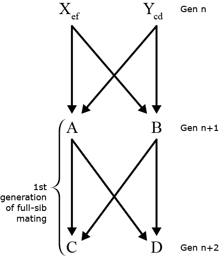
Full-Sib Mating (1)
Fig.3 and schematic of Full-sib mating design, from generation n to generation n+ 2
Probability that A & B both receive e from X =
[latex]({1 \over 2})({1 \over 2}) = {1 \over 4}[/latex]
Probability that A & B both receive f from X =
[latex]({1 \over 2})({1 \over 2}) = {1 \over 4}[/latex]
Probability that e and f are not IDB =
[latex]1-F_x[/latex]
Probability that A & B contain an identical allele from X by chance (given that e and f are not IBD) =
[latex]({1 \over 4}+{1 \over 4} )(1 - F_x)[/latex]
[latex]\textrm{Equation 10}[/latex] Formula for calculating probability that an allele in A and B form parent X is IBD knowing that alleles e and f in X are not IBD.
where:
[latex]F_{x}[/latex] = the coefficient of inbreeding of X, i.e., the probability that e and f are IBD.
Full-Sib Mating (2)
Probability that e and f are identical =
[latex]F_x[/latex]
Probability A & B receive an identical allele from X (given that e and f are IBD) = 1
Total probability that A & B receive an identical allele from X, and from Y can be determined using Equation 11.
[latex]F_x + {1\over 2}(1 - F_x) = {1\over 2}(1 + F_x) = r_{xx}, \; and\; F_y + {1\over 2}(1 - F_y) = {1\over 2}(1 + F_y) = r_{yy}[/latex]
[latex]\textrm{Equation 11}[/latex] Formula for calculating the probability that progenies A and B received identical alleles from parents X and Y,
where:
[latex]r_{xx}, r_{yy}[/latex] = the probability of identical alleles from either parent,
[latex]F_x[/latex] = the coefficient of inbreeding of x,
[latex]F_y[/latex] = the coefficient of inbreeding of y.
Full-Sib Mating (3)
Let us consider full-sib mating where the relationship between genes in offspring from the two parents can be represented by Equation 12.
[latex]r_{AB} = {1 \over 4}[r_{xx} + 2r_{xy} + r_{yy}][/latex]
[latex]\textrm{Equation 12}[/latex] Formula for calculating the probability that a gene from parent X to progeny A, and from parent Y to progeny B are IBD.
where:
[latex]\textrm{terms}[/latex] are as described below.
Probability that a gene from X to A and one from Y to B are IBD is [latex]r_{xy}[/latex].
Probability that a gene from Y to A and one from X to B are IBD is [latex]r_{xy}[/latex].
Full-Sib Mating (4)
The relationship between X and Y, rxy, could be zero if the reference population from which X and Y are sampled is considered to be random mating and large. Note that if the population is random mating but is not large, then the relationship coefficient may not be zero. The relationship can be represented as in Equation 13.
[latex]F_{xy} = F_y = F_n, \;and\; \large r_{xy} = r_n[/latex]
[latex]\textrm{Equation 13}[/latex] Formula for calculating the relationship between two parents.
where:
[latex]\textrm{terms}[/latex] have been defined previously.
In the form represented in Equation 13, notice that the relationship between X and Y is equal to the average relationship in the nth generation of random mating and the series of equations in Equation 14 shows the relationships in progression.
[latex]r_{n+1} = {1 \over 4} [r_{xx} + r_{yy} +2r_{xy}][/latex]
[latex]= {1 \over 4} [{1 \over 2} (1 + F_n) + {1 \over 2} (1 + F_n) + 2r_n][/latex]
[latex]r_{n+1} = F_{n+2}[/latex]
[latex]r_n = F_{n+1}[/latex]
[latex]F_{n+2} = r_{n+1} = {1 \over 4} [{1 \over 2} (1 + F_n) + {1 \over 2} (1 + F_n) + 2F_{n+1}][/latex]
[latex]= {1 \over 4} [1 + F_n + 2F_{n+1}][/latex]
[latex]P_{n+2} = {1 \over 2} P_{n+1} + {1 \over 4} P_n[/latex]
[latex]F_n = 1 - ({1 \over 2})^n (1- F_0)[/latex]
[latex]\textrm{Equation 14}[/latex] Formula for calculating the relationship between two parents in different generations of random mating.
where:
[latex]\textrm{terms}[/latex] are as defined previously.
Self-Pollination
Assume original population is non-inbred (by definition = F2). Using Equation 9 the relationship between the panmictic index and the coefficient of relationship can be calculated for different generations of self pollination assuming the original population is non-inbred (by definition = F2) (Table 2). Where:
[latex]P_n = ({1 \over 2})^nP_0,\;and\;F = {1 \over 2}\left[ 1+ F_x\right][/latex].
| Generation | P | F |
|---|---|---|
| 0 | 1.00000000 | 0.00000000 |
| 1 | 0.50000000 | 0.50000000 |
| 2 | 0.25000000 | 0.75000000 |
| 3 | 0.12500000 | 0.87500000 |
| 4 | 0.06250000 | 0.93750000 |
| 5 | 0.03125000 | 0.98437500 |
| 6 | 0.01562500 | 0.98437500 |
| 7 | 0.00781250 | 0.99218750 |
| 8 | 0.00390625 | 0.99609375 |
| 9 | 0.00195313 | 0.99804688 |
| 10 | 0.00097656 | 0.99902344 |
 |
0.00000000 | 1.00000000 |
Full-Sibing
In a similar manner, the relationship between the panmictic index and the coefficient of relationship can be calculated for different generations for full-sib mating situation as shown in Table 3, where:
[latex]P_{n+2} = {1 \over 2}P_{n+1} + {1 \over 4}P_n[/latex]
| Generation | P | F |
|---|---|---|
| 0 | 1.00000000 | 0.00000000 |
| 1 | 1.00000000 | 0.00000000 |
| 2 | 0.75000000 | 0.25000000 |
| 3 | 0.62500000 | 0.37500000 |
| 4 | 0.50000000 | 0.50000000 |
| 5 | 0.40625000 | 0.59375000 |
| 6 | 0.32812500 | 0.73437500 |
| 7 | 0.26562500 | 0.78515625 |
| 8 | 0.21484375 | 0.78515625 |
| 9 | 0.17382813 | 0.82617188 |
| 10 | 0.14062500 | 0.85937500 |
|
0.00000000 | 1.00000000 |
References
Emik, l. O., and C. E. Terrill. 1949. Systematic procedures for calculating inbreeding coefficients. J. Heredity, 40 (2): 51–55.
Cockerham, C. C. 1971. Higher order probability functions of identity of alleles by descent. Genetics 69:235–246.
How to cite this chapter: Beavis, W., K. Lamkey, and A. A. Mahama. 2023. Resemblance Between Relatives. In W. P. Suza, & K. R. Lamkey (Eds.), Quantitative Genetics for Plant Breeding. Iowa State University Digital Press.
