
Chapter 6: Components of Variance
William Beavis; Kendall Lamkey; Katherine Espinosa; and Anthony Assibi Mahama
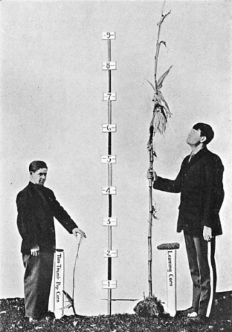
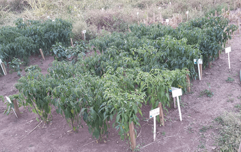
This chapter explores sources of phenotypic variation (Fig. 1), whether genetic or environmental and how these contribute to the heritability of selected traits. It covers the derivation of variance components and covariance, the relationship among variance components, and the role of epistasis.
Type your learning objectives here.
- Learn to model components of genetic variances for purposes of estimating heritability.
- Be able to explain:
- The impact of allele frequencies on genetic components of genotypic variability,
- The reason estimates of components of genetic variability are limited to the population from which they are estimated,
- The reason additive variance does not imply additive gene action and
- How additive genetic variance can arise from genes with any degree of dominance or epistasis.
Phenotypic Components of Variance
Recall that our working model for the phenotype includes genotypic and non-genotypic (environmental) sources of variability (Equation 1):
[latex]P = \mu + G + E[/latex]
[latex]\textrm{Equation 1}[/latex] Working model of phenotypic, genotypic, and environmental effects,
where:
[latex]\mu[/latex] = overall mean,
[latex]G[/latex] = genotypic effect,
[latex]V_{E}[/latex] = environmental effect.
The source of phenotypic variability determines whether selection for the trait will result in a heritable response, i.e., will be passed on to the next generation.
For purposes of making decisions in plant breeding, if two populations have different phenotypic means, we want to know whether the differences are due to different environments, different genotypes, or some combination of both. If the differences are due to genotypic differences, then what proportion of the genotypic differences is heritable?
Algebraic Description
Using simple algebra and our working model, we can show that the phenotypic variance VP within a population is equal to the sum of the genotypic variance VG and environmental variance VE, assuming that VG and VE are independent (Equation 2);
[latex]V(P)=V(G) + V(E)[/latex]
[latex]\textrm{Equation 2}[/latex] Working model of phenotypic, genotypic, and environmental variances,
If the genotypic values and environmental deviations are not independent, the V(P)=V(G+E), and V(P) can be increased by twice the covariance of G with E if they are not independent (Equation 3):
[latex]V(P) = V(G) +V(E) + 2Cov(G,E)[/latex]
[latex]\textrm{Equation 3}[/latex] Composition of phenotypic variance,
where:
[latex]Cov(G,E)[/latex] = joint variation between G and E.
Genetic Components of Variance
Genetic components of variability can be divided into several subcategories, including additive variance, VA, dominance variance, VD, and epistatic variance, VI. Together, the values for each of these subcategories yield the total amount of genetic variation, VG, responsible for a particular phenotypic trait: VP = VG + VE.
Consider the ratio of VG to VP. This was originally recognized by statistical geneticists (such as RA Fisher) as the genotypic intra-class correlation. To understand this, consider the evaluation of a line i, for a phenotype, Y. Next, imagine that you can evaluate line i repeatedly. Let us designate these repeated measurements as j. We can then designate these repeated measurements of the phenotype as Yij. There is a Covariance among these repeated evaluations that we can represent as [latex]Cov(Yij, Yij')= Var(Gi), for\; j\neq{j'})[/latex].
Explanation of Formula
Thus the correlation among these repeated measures is (Equation 4)
[latex]\rho(Y_{ij},Y_{ij'}) = \frac{Cov(Y_{ij}, Y_{i,j'})}{\sqrt{Var{(Y_{ij})Var{(Y_{ij'})}}}}[/latex],
[latex]\textrm{Equation 4}[/latex] Correlation among repeated measures,
where:
[latex]\rho[/latex] = correlation between Yij and Yij’,
[latex]Cov(Y_{ij}, Y_{i,j'})[/latex] = covariance between Yij and Yij’,
[latex]Var({Y_{ij}})[/latex] & [latex]Var({Y_{ij'}})[/latex] = variance ofYij and Yij’.
Because [latex]Var(Y_{i,j}) = V(G_i)+V(E_{ij})[/latex], the correlation is represented by Equation 5.
[latex]\rho(Y_{ij},Y_{ij'}) = \frac{V(G_i)}{V(G_i)+V(E_{ij})} = \frac{V(G_i)}{V(P_{ij})}[/latex]
[latex]\textrm{Equation 5}[/latex] Correlation among repeated measures,
where:
[latex]\rho[/latex] = correlation between Yij and Yij’,
[latex]V(G_{i}[/latex] = genotypic variance of genotype i,
[latex]Var({E_{ij}})[/latex] = variance of environment j for genotype i,
[latex]Var({P_{ij}})[/latex] = phenotypic variance of genotype i in environment j.
Heritability in the Broad Sense
Broad sense heritability is estimated by Equation 6.
[latex]H= \frac{V_{G}}{V_{P}}[/latex]
[latex]\textrm{Equation 6}[/latex] Formula for estimating broad sense heritability,
where:
[latex]V_{G}[/latex] = the total genetic variance,
[latex]V_{P}[/latex] = the phenotypic variance.
JL Lush, an animal breeder, also referred to this intra-class correlation coefficient as heritability in the broad sense (1937). He wanted to distinguish the application of intra-class correlation to animals from the concept of repeatability. Repeatability as an engineering concept refers to the same measurement procedure conducted by a single observer, using a single measuring instrument, under the same conditions, at a single location, over a short period of time. As a result, plant and animal breeders tend to prefer the use of broad sense heritability for the genotypic intra-class correlation, although both plant and animal breeders routinely evaluate a single trait on individual genotypes repeatedly over time and space (locations and years).
Broad-Sense Components
The genetic variance can be recognized as consisting of several components (Equation 7):
[latex]V_{G} = V_{A} + V_{D} + V_{I}[/latex]
[latex]\textrm{Equation 7}[/latex] Composition of total genotypic variance,
where:
[latex]V_{G}[/latex] = total genotypic variance,
[latex]V_{A}[/latex] = additive genetic variance, that is, the variance of breeding values, and refers to the deviation from the mean phenotype due to inheritance of a particular allele and this allele’s relative effect on phenotype, i.e., relative to the mean phenotype of the population,
[latex]V_{D}[/latex] =dominance variance due to interactions between alternative alleles at a specific locus,
[latex]V_{I}[/latex] = epistatic variance due to interaction between alleles at different loci.
Heritability in the Narrow Sense
Heritability in the narrow sense was defined by JL Lush (1937) to represent the extent to which phenotypes are determined by the genes transmitted from their parents (Equation 8):
[latex]h^{2} = \frac{V_{A}}{V_{P}}[/latex]
[latex]\textrm{Equation 8}[/latex] Composition of total genotypic variance,
where:
[latex]h^{2}[/latex] = heritability in the narrow sense,
[latex]V_{A}[/latex] = additive genetic variance, that is, the variance of breeding values, and refers to the deviation from the mean phenotype due to inheritance of a particular allele and this allele’s relative effect on phenotype, i.e., relative to the mean phenotype of the population,
[latex]V_{P}[/latex] = phenotypic variance.
So, we can now expand our model for the phenotypic variance to include several genetic variance components and environmental variance as in Equation 9.
[latex]V_{P} = V_{A} + V_{D} + V_{I} + V_{E}[/latex]
[latex]\textrm{Equation 9}[/latex] Composition of total genotypic variance,
where:
[latex]V_{E}[/latex] = environmental variance. Other variables are as described previously.
| Variance component | Symbol | Source of variation |
| Phenotypic | [latex]V_{P}[/latex] | Phenotypic value |
| Genotypic | [latex]V_{G}[/latex] | Genotypic Value |
| Additive | [latex]V_{A}[/latex] | Breeding Value |
| Dominance | [latex]V_{D}[/latex] | Dominance deviation |
| Interaction | [latex]V_{I}[/latex] | Interaction deviation |
| Environmental | [latex]V_{E}[/latex] | Non-genetic deviation |
Deriving Variance Components
The genetic components of variance are influenced by the gene frequency and the assigned genotypic values[latex]a[/latex] and [latex]d[/latex]. The information needed to derive [latex]V_{A}[/latex] and [latex]V_{D}[/latex] are:
| Genotypes | [latex]AA[/latex] | [latex]Aa[/latex] | [latex]aa[/latex] |
|---|---|---|---|
| Frequencies | [latex]p^{2}[/latex] | [latex]2pq[/latex] | [latex]q^{2}[/latex] |
| Coded GV | [latex]a[/latex] | [latex]d[/latex] | [latex]-a[/latex] |
| Genotypic Value | [latex]2q(a-pd)[/latex] [latex]2q(a-qd)[/latex] |
[latex]a(q-p) + d(1-2pq)[/latex] [latex](q-p)a + 2pqd[/latex] |
[latex]-2p(a+qd)[/latex] [latex]-2p(a+pd)[/latex] |
| Breeding Value | [latex]2qa[/latex] | [latex](q-p)a[/latex] | [latex]-2pa[/latex] |
| Dominance Deviation | [latex]-2q^{2}d[/latex] | [latex]2pqd[/latex] | [latex]-2p^{2}d[/latex] |
The variances are thus obtained by squaring the values in the table, multiplying by the frequency of the genotype concerned, and summing over the three genotypes (Equation 10).
[latex]\eqalign {V_A &= 4p^2q^2\alpha^2 + 2pq{(q-p)}^2\alpha^2 + 4p^2q^2\alpha^2 \\ &= 2pq(2pq + q^2-2pq+p^2+2pq)\alpha^2 \\ &= 2pq(p^2+2pq+q^2)\alpha^2 \\ &= 2pq\alpha^2 \\ &= 2pq[a+d(q-p)]^2 \\ V_D &= d^2(4q^4p^2+ 8p^3q^3+4p^4q^2) \\ &= 4p^2q^2d^2(q^2+2pq+p^2) \\ &= (2pqd)^2 }[/latex]
[latex]\textrm{Equation 10}[/latex] Derivation of additive and dominance variances,
where:
[latex]p[/latex] = frequency of allele [latex]A[/latex],
[latex]q[/latex] = frequency of allele [latex]a[/latex],
[latex]\alpha[/latex] = average effect of an allele,
[latex]a, d[/latex] = coded genotypic values.
Covariance
If there is no dominance at the locus under consideration d = 0, then: [latex]V_{A} = 2pq\alpha^2[/latex].
If there is complete dominance d = a, the additive variance becomes [latex]V_{A} = 8pq^3\alpha^2[/latex].
The total genetic variance is estimated with Equation 11.
[latex]V_{G} = V_A + V_D + 2COV_{AD}[/latex]
[latex]\textrm{Equation 11}[/latex] Total genetic variance formula including covariance of additive and dominance variances,
where:
[latex]COV_{AD}[/latex] is the covariance of breeding values with dominance deviations, which can be demonstrated to be zero. Thus substituting in Equation 12,
[latex]V_G = V_A + V_D = 2pq[a+d(q-p)]^2 + [2pqd]^2[/latex]
[latex]\textrm{Equation 12}[/latex] Total genetic variance formula relating additive and dominance variances to allele frequencies and coded genotypic values,
where:
[latex]V_A, V_D, p, q, and, d[/latex] are as described previously.
Component Relationships
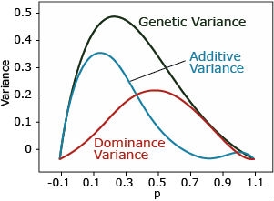
The relationships among variance components, gene action, and allele frequencies for the two allele case can be graphically represented (Figs. 3, 4, 5).
Additive Gene Action
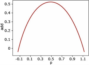
Additive gene action: There is no dominance (a>0, d=0). In this case, the genetic variance is additive, and it is greatest when p=q=0.5.
Complete Dominance
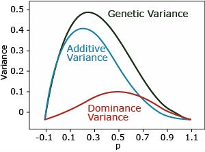
Complete dominance: ([latex]a > 0, d = a[/latex]). The dominance variance is maximal when p=q=0.5. The additive is maximal when p=0.3.
Overdominance
Overdominance: ([latex]a = 0, d > 0[/latex]). The dominance variance is the same as incomplete dominance.
Important principles to remember:
- All the components of genetic variance are dependent on the gene frequencies.
- Estimates of components of genetic variances are valid only for the population from which they are estimated.
- The concept of additive variance does not carry with it the assumption of additive gene action; the existence of additive variance is not an indication that genes act additively.
- Additive variance can arise from genes with any degree of dominance or epistasis.
Influence of Epistasis
Two Or More Loci: Influence of Epistasis on Components of Genetic Variance
When more than one locus is under consideration, then deviations due to interactions among loci give rise to additional variance components due to epistatic interactions, Vi (Equation 13).
[latex]V_I = V_{AA} + V_{AD} + V_{DD} + etc.[/latex]
[latex]\textrm{Equation 13}[/latex] Components of epistatic interaction variance,
where:
[latex]V_{AA}[/latex] = additive × additive variance is the interaction between two breeding value,
[latex]V_{AD}[/latex] = additive × dominance variance is the interaction between the breeding value of one locus and the dominance deviation of the other,
[latex]V_{DD}[/latex] = dominance × dominance variance is the interaction between the two dominance deviations.
Epistatic Model
A non-intuitive consequence of the epistatic models is that additive variance can arise from purely epistatic genetics. For example, let’s consider the special case of an F2 population with equal frequencies of two alleles at each of two independently segregating loci. Let’s imagine that we know the genotypes at each of these functional loci and analyze the F2 population using a regression approach for each of the loci and their interactions.
| Source of variance | Df |
| Locus A | 2 |
| Linear (Additive) | 1 |
| Quadratic (Dominance) | 1 |
| Locus B | 2 |
| Linear (Additive) | 1 |
| Quadratic (Dominance) | 1 |
| Epistasis | 4 |
| Linear A x Linear B (A * A) | 1 |
| Linear A x Quadratic B (A * D) | 1 |
| Quadratic A x Linear B (D * A) | 1 |
| Quadratic A x quadratic B (B * D) | 1 |
| Total | 8 |
Example 1
Analysis of a phenotype in an F2 population with equal frequencies of alleles at two functionally polymorphic loci, each contributing only additive coded genotypic values from the A locus and a B locus, i.e., [latex]P=\mu + a_{A} + a_{B}[/latex], where [latex]\mu[/latex]= 5, [latex]a_{A}[/latex] = 3, and [latex]a_{B}[/latex] =1.
| Parameter | Value |
| [latex]a_{A}[/latex] | 3 |
| [latex]d_{A}[/latex] | 0 |
| [latex]a_{B}[/latex] | 1 |
| [latex]d_{B}[/latex] | 0 |
| [latex]\mu[/latex] | 5 |
| n/a | n/a | [latex]A_{1}A_{1}[/latex] | [latex]A_{1}A_{2}[/latex] | [latex]A_{2}A_{2}[/latex] | Mean |
| n/a | n/a | 1/4 | 1/2 | 1/4 | n/a |
| [latex]B_{1}B_{1}[/latex] | 1/4 | 9 | 6 | 3 | 6 |
| [latex]B_{1}B_{2}[/latex] | 1/2 | 8 | 5 | 2 | 5 |
| [latex]B_{2}B_{2}[/latex] | 1/4 | 7 | 4 | 1 | 4 |
| Mean | n/a | 8 | 5 | 2 | 2.75 |
| Variance component | Variance |
| [latex]\delta^2_{A_A}[/latex] | 4.5 |
| [latex]\delta^2_{A_B}[/latex] | 0.5 |
| [latex]\delta^2_{D_A}[/latex] | 0 |
| [latex]\delta^2_{D_B}[/latex] | 0 |
| [latex]\delta^2_{AA}[/latex] | 0 |
| [latex]\delta^2_{AD}[/latex] | 0 |
| [latex]\delta^2_{DA}[/latex] | 0 |
| [latex]\delta^2_{DD}[/latex] | 0 |
Example 2
Analysis of a phenotype in an F2 population with equal frequencies of alleles at two functionally polymorphic loci where only single epistatic interaction between the genotypes will produce an altered phenotype, [latex]P=\mu + a_{A} + a_{B} + d_{A} + d_{B} + e_{AABB}[/latex], where [latex]\mu[/latex] = 0, [latex]a_{A}[/latex] = 0, [latex]a_{B}[/latex] = 0, [latex]d_{A}[/latex] = 0, [latex]d_{B}[/latex] = 0, [latex]d_{AABB}[/latex] = 50.
| n/a | n/a | [latex]A_{1}A_{1}[/latex] | [latex]A_{1}A_{2}[/latex] | [latex]A_{2}A_{2}[/latex] | Mean |
| n/a | n/a | 1/4 | 1/2 | 1/4 | n/a |
| [latex]B_{1}B_{1}[/latex] | 1/4 | 0 | 0 | 0 | 0 |
| [latex]B_{1}B_{2}[/latex] | 1/2 | 0 | 0 | 0 | 0 |
| [latex]B_{2}B_{2}[/latex] | 1/4 | 0 | 0 | 50 | 12.5 |
| Mean | n/a | 0 | 0 | 12.5 | 3.125 |
| Population variances | Population | Percent |
| Total genetic | 146.484 | 100.0% |
|
Additive effects |
39.063 | 26.7% |
|
Dominance |
19.531 | 13.3% |
|
Epistasis |
87.891 | 60.0% |
References
Lush J. L. 1937. Animal Breeding Plans, Collegiate Press Inc, Ames, IA.
How to cite this chapter: Beavis, W., K. Lamkey, K. Espinosa, and A. A. Mahama. 2023. Components of Variance. In W. P. Suza, & K. R. Lamkey (Eds.), Quantitative Genetics for Plant Breeding. Iowa State University Digital Press.
