Selection is the crux of crop improvement and makes use of the art and science concepts to ensure the success (gains derived) of a breeding program or specific project. This chapter explains principles and practices related to genetic gain.

Underlying Theory of Selection

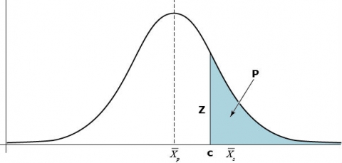
Let [latex]\bar{X_p}[/latex] be the mean phenotypic value of a quantitative trait that is normally distributed in a large random mating population (Fig. 1). Also, designate [latex]\bar{X_s}[/latex] as the mean of a selected proportion P of this population, where c is the truncation point of selection and Z is the height of the ordinate at the selection truncation point.

The selection differential is defined as in Equation 1:

[latex]S = \bar{X}_s - \bar{X}_p[/latex].

[latex]\textrm{Equation 1}[/latex] Formula for calculating selection differential.

where:
[latex]S[/latex] = selection differential,
[latex]\bar{X}_s[/latex] = mean of selected proportion,
[latex]\bar{X}_p[/latex] = mean of the population.

If [latex]\sigma^2_p[/latex]is the phenotypic variance in the population, then the standardized selection differential can be written as in Equation 2:

[latex]\large i=\frac{S}{\sigma_p}=\frac{\bar{X}_s - \bar{X}_p}{\sigma_p}[/latex].

[latex]\textrm{Equation 2}[/latex] Formula for calculating standardized selection differential.

where:
[latex]i[/latex] = standardized selection differential; also, is the number of standard deviations represented by the selection differential, S,
[latex]\sigma_p[/latex] = square root of phenotypic variance in the population,
[latex]\bar{X}_s[/latex] = mean of selected proportion,
[latex]\bar{X}_p[/latex] = mean of the population.

Selection Response

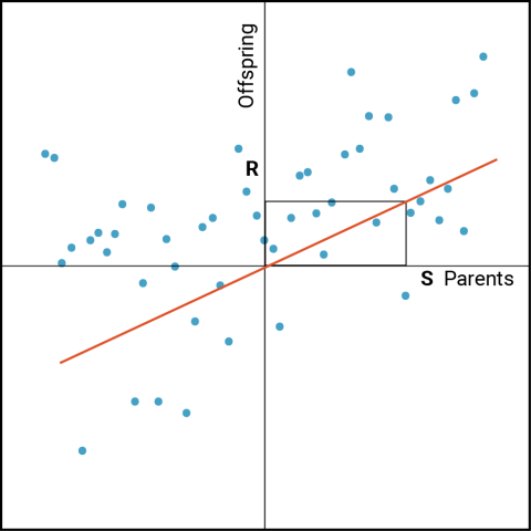
While [latex]\bar{X_s}[/latex]may be distinctive relative to [latex]\bar{X_p}[/latex] , of greater interest are the phenotypes of the progeny derived from crosses among the selected parents [latex]\bar{X_s}[/latex]. The predicted response of progeny to the selection of their parents can be derived from the relationship between parent and offspring as follows (Fig. 2). Designate R as the response to selection measured in the offspring (represented as a deviation from the population mean). S is the selection differential (represented as a deviation from the population mean) as described in the previous section.

Genetic Gain

The response to selection ( R ) can be written simply as in Equation 3:

[latex]R=b_{o\bar{p}}S[/latex].

[latex]\textrm{Equation 3}[/latex] Formula for calculating response to selection.

where:
[latex]R[/latex] = response to selection,
[latex]b_{o\bar{p}}[/latex] = the regression coefficient of offspring on the mid-parent value,
[latex]S[/latex] = the selection differential.

The regression coefficient of offspring on the mid-parent value can be written as in Equation 4:

[latex]\large b_{o\bar{p}} = \frac{Cov(o,\bar{p})}{Var(\bar{p})} = \frac{Cov(o,\bar{p})}{\frac{1}{2}\sigma^2_P}[/latex]

[latex]\textrm{Equation 4}[/latex] Formula for calculating the regression coefficient.

where:
[latex]Cov(o,\bar{p})[/latex] = the covariance of offspring on mean of parents,
[latex]Var(\bar{p})[/latex] = the variance of mid-parent,
[latex]\sigma^2_P[/latex] = the phenotypic variance.

Equation 4 is written that way because:

[latex]Var({\bar{p}}) = Var(\frac{P_m+P_f}{2}) = \frac{1}{4}Var(P_m + P_f) = \frac{1}{2}{\sigma^2_P}[/latex]

[latex]\textrm{Equation 5}[/latex] Formula for calculating the mean of parent phenotype.

where:
[latex]P_{m}[/latex] = the phenotype of the male parent,
[latex]P_{f}[/latex] = the phenotype of the female parent.

Also, we can show that: [latex]Cov(o,\bar{p}) = \frac{1}{2}\sigma_A^2,\textrm{so} \ b_{\bar{OP}} = \frac{ \frac{1}{2}\sigma_A^2}{ \frac{1}{2}\sigma_P^2} = \frac{ \sigma_A^2}{ \sigma_P^2} = h^2[/latex]

Therefore, R is written as in Equation 6:

[latex]\large R = h^2S = ih^2\sigma_p = \Delta G_c[/latex]

[latex]\textrm{Equation 6}[/latex] Formula for calculating the change in genetic gain.

where:
[latex]\Delta G_c[/latex] = the rate of genetic gain per cycle,
[latex]h^2[/latex] = the narrow sense heritability,
[latex]\sigma_{p}[/latex] = the standard deviation of the phenotype,
[latex]\textrm{other terms}[/latex] are as defined previously.

R is the selection response or Genetic Gain, as Lush defined it in 1940. This equation for ΔG, also known as the Breeder’s Equation, based on the regression of offspring values on mid-parent values, is difficult to apply directly to plant breeding systems because plant breeders typically evaluate hundreds of replicated individuals representing thousands of genotypes grown in replicated plots in dozens to hundreds of environments. Unlike most animal systems, it is possible to replicate progeny genotypes due to the diversity of reproductive biology that is available to plant breeders: clonal propagation, doubled haploids, and tolerance to inbreeding through self-pollinations for multiple generations. In the last example, the response units can be several generations removed from the parental (crossing) generation. The type of reproductive biology will affect the details of how we estimate the response to selection, ΔG_c, also referred to as the “Rate of Genetic Gain”, per cycle.

Heritability on an Entry-Mean Basis

Recall plant breeders often report heritability from field experiments on an entry-mean basis represented as in Equation 7:

[latex]H= \large \frac{\sigma^2_{G}}{\sigma^2_{G}+\left( \frac{\sigma^2_{GE}}{E} \right)+\left( \frac{\sigma^2_{\varepsilon}}{rE} \right)}[/latex]

[latex]\textrm{Equation 7}[/latex] Formula for calculating heritability on entry mean basis.

where:
[latex]\sigma^2_{G}[/latex] = the genotypic variance,
[latex]\sigma^2_{GE}[/latex] = the genotype by environment variance,
[latex]\sigma^2_{\varepsilon}[/latex] = the residual or error variance,
[latex]r[/latex] = the number of replications
[latex]E[/latex] = number of environments.

Although Equation 7 is similar to Lush’s broad sense heritability, it is not exactly the same concept because it can be ‘adjusted’ by adding replicates and environments to reduce the impact of σ²_GE and [latex]\varepsilon[/latex] on the estimated phenotypic variance.

The problem for plant breeders is that the concept of evaluating individual plants and the performance of their progeny to obtain an estimate of heritability simply is of no practical use for most crops where plot performance is the basis for selection. Hanson attempted to address this by framing the multiple concepts of heritability within the context of genetic gain (1963).

Hanson defined heritability as “the fraction of the selection differential expected to be gained when selection is practiced on a defined reference unit.” Given the standard definition for selection response is [latex]\Delta G=i\frac{\sigma^2_{G}}{\sigma^2_{\bar{y}}}\sigma_{\bar{y}}=ih^{2}\sigma_{\bar{y}}=R[/latex], we can then solve for h² using the expression in Equation 8:

[latex]h^{2}=\large \frac{R}{i\sigma_{\bar{y}}}[/latex]

[latex]\textrm{Equation 8}[/latex] Formula for estimating realized heritability,

where:
[latex]\textrm{terms}[/latex] are as defined previously.

That is the standardized response to selection or realized heritability.

Context of Heritability

Within the framework of genetic gain, Hanson defined heritability in such a manner as to be consistent with the original concept while at the same time taking into consideration that it has little meaning unless the selection units (entry means) and response units are defined. Thus, when plant breeders wish to communicate information about heritability, they should specify:

1. A reference population of genotypes.
2. A reference population of environments. i.e., the target environments.
3. Selection units
4. Response units

This context emphasizes the purpose of obtaining variance component estimates, usually for the purpose of comparing genetic gains (ΔG) under various possible breeding procedures. The results are used to make decisions about which procedure to employ. Indeed, it is in this context that variance components of heritability are used as “plug-in values” (Sprague and Eberhart, 1977) for a six-step decision-making algorithm that uses ΔG as an arbiter for comparing breeding methods (Fehr, 1994; Chapter 17). Actually, this back-of-the-envelope algorithm is fairly insensitive to the estimated heritability values, and there are more effective means of optimizing genetic gain, number of generations, and costs.

Family Structure

Assume our selection and response units are represented by some family structure, say half-sibs, or full-sibs, or recombinant inbred lines, as examples. Also, recall that we can equate the genotypic variance component, designated as f for family relationships, to the genetic covariance of relatives. Thus, the Cov(R,S) = Var(f). Also, note that the Var(S) is the phenotypic variance among the entry means. Thus, B_SR is the proportion of variance among family units relative to the phenotypic variance among entry means. We might refer to this as the heritability of the family units represented in Equation 9:

[latex]h^2_f =\large \frac{\sigma^2_f}{\sigma^2_p}[/latex]

[latex]\textrm{Equation 9}[/latex] Formula for estimating heritability of family units,

where:
[latex]\sigma^2_{f}[/latex] = the family unit variance,
[latex]\sigma^2_{P}[/latex] = the phenotypic variance.

If the replicated plots consist of half-sibs from a random mating population, then the variance component among half-sibs on an entry mean basis is equal to the covariance of the half-sibs (Equation 10), ignoring epistasis:

[latex]Cov(HS)=\frac{1}{4}\left( 1+F \right)\sigma^2_A[/latex]

[latex]\textrm{Equation 10}[/latex] Formula for estimating covariance of half-sibs, ignoring epistasis,

where:
[latex]F[/latex] = the inbreeding coefficient
[latex]\sigma^2_{A}[/latex] = the additive variance.

Narrow-Sense Heritability of Half-Sibs

Thus, it is possible to utilize the estimated variance components from an ANOVA to estimate a “narrow sense heritability”, h², by simply multiplying this variance component by 4/(1+F) and plugging the value into Equation 7 as in Equation 11; all terms are as defined previously:

[latex]h^2=\large \frac{\sigma^2_{A}}{\sigma^2_{G}+\left( \frac{\sigma^2_{GE}}{E} \right)+\left( \frac{\sigma^2_{e}}{rE} \right)}[/latex]

[latex]\textrm{Equation 11}[/latex] Formula for estimating narrow sense heritability of half-sibs.

Notice that this is not the same as the original narrow sense heritability as defined by Lush (1940), but is a narrow sense heritability for a population of half-sibs.

Next, consider the numerator in Equation 11 above. In the case of half-sibs, we have learned that the variance of family units is represented as in Equation 12.

[latex]\sigma^2_f = Cov(HS) = \sigma_{HS} = \frac{(1+F)}{4}\sigma^2_A + \Bigg[\frac{(1+F)}{4} \Bigg]^2\sigma^2_{AA}+ \dots[/latex]

[latex]\textrm{Equation 12}[/latex] Alternative formula for estimating family units variance,

where:
[latex]\sigma^2_{AA}[/latex] = the additive by additive interaction variance.

Covariance Estimation

Again, if the data are not balanced, the variance component will not be estimated correctly unless REML is used. Let us assume that we obtain a ‘best’ estimate for σ_HS, either because our data are balanced or we have used REML. Should we use the previous equation for the Cov(R,S)? To answer this, we have to recognize that there is a genetic relationship between selection units and response units, i.e., there is a pedigree relationship or coefficient of coancestry between the selection and response units, and Equation 12 does not take this into consideration. In the case where both selection units and response units are half-sibs, the Cov(R,S) is represented as in Equation 13

[latex]Cov(R,S) = \frac{(1+F)}{4}\sigma^2_A + \frac{1}{32}[1+F]^2\sigma^2_{AA}+ \dots[/latex]

[latex]\textrm{Equation 13}[/latex] Formula for estimating covariance of response units and selection units,

where:
[latex]\textrm{terms}[/latex] are as defined previously.

Note that if Equation 13 is used, a slightly biased estimate of heritability will result even if the best estimates of variance components are obtained. This is due to epistatic variance. For other types of progeny, the bias in the numerator can be much larger. Let us look at estimates based on Equation 13 for some example cases/progeny types.

Example A

Estimation of Narrow sense heritability from a half-sib family experiment with data obtained on individual plants in one environment.

1. Heritability on an individual plant basis

• • Selection among individual plants
  • 1 Replication in 1 environment
  • Response is measured in outbred progeny

[latex]Example\ A \\ \large\eqalign{h^2_1 &= \frac{(\frac{4}{1+F_P}){\hat\sigma^2_F}}{{\hat\sigma^2_p}} = \frac{{\hat\sigma^2_A}+(\frac{1+F_P}{4}){\hat\sigma^2_{AA}}}{{\hat\sigma_p^2}}\\ {\hat\sigma^2_p} &= {\hat\sigma^2_F}+ {\hat\sigma^2_{FE}} + {\hat\sigma^2_\epsilon} + {\hat\sigma^2_\omega} \\ Bias &= \frac{\frac{1}{4}(F_p - 1)\sigma^2_{AA}}{\sigma^2_p}\\ \sigma^2_F &= \frac{(1+F_p)}{4}\sigma^2_A + \frac{(1+F_P)^2}{16}\sigma^2_{AA}}[/latex]

where: [latex]\hat\sigma^2_{FE}[/latex] is the estimated family by environment interaction variance; [latex]\hat\sigma^2_\epsilon[/latex] is the estimated error variance, and [latex]\hat\sigma^2_\omega[/latex] is the estimated within family variance.

Example B

Estimation of Narrow sense heritability from a half-sib family experiment with data obtained on individual plants in multiple independent environments.

2. Family heritability on a plot basis (half-sib family, single plot mean values)

• • Selection among plot means
  • 1 Replication in 1 environment
  • Response is measured in outbred progeny

[latex]Example\ B \\ \large\eqalign{h^2_1 &= \frac{\hat{\sigma}^2_F}{\hat{\sigma}^2_p} = \frac{\frac{1}{4}(1+F_p)\hat{\sigma}^2_A+\frac{1}{16}(1+F_p)^2\,\hat{\sigma}^2_{AA}}{\hat{\sigma}^2_p} \\ \hat{\sigma}^2_p &= \hat{\sigma}^2_F+ \hat{\sigma}^2_{FE} + \hat{\sigma}^2_\epsilon + \frac{\hat{\sigma}^2_\omega}{n} \\ Bias &= \frac{\frac{1}{32}(1+F_p)^2\hat{\sigma}^2_{AA}}\, {\sigma^2_p} \\ \hat{\sigma}^2_F &= \frac{(1+F_p)}{4}\sigma^2_A + \frac{(1+F_p)^2}{16}\sigma^2_{AA} }[/latex]

where: [latex]n[/latex] is the number of entries or plots; all other terms are described in example A.

Computational Considerations

Example C

Estimation: Narrow sense heritability estimated from a half-sib family experiment with data obtained on individual plants in multiple independent environments.

3. Family heritability

• • selection among half-sib family mean averaged over environments
  • outbred progeny

[latex]Example\ C \\ \large \eqalign{h^2_1 &= \frac{\hat{\sigma}^2_F}{\hat{\sigma}^2_p} = \frac{\frac{1}{4}(1+F_p)\hat{\sigma}^2_A+\frac{1}{16}(1+F_p)^2\hat{\sigma}^2_{AA}}{\hat{\sigma}^2_p} \\ \hat{\sigma}^2_p &= \hat{\sigma}^2_F+\frac{ \hat{\sigma}^2_{FE}}{e} +\frac{ \hat{\sigma}^2_\epsilon}{er} + \frac{\hat{\sigma}^2_\omega}{ern} \\ Bias &= \frac{\frac{1}{32}(1+F_P)^2\hat{\sigma}^2_{AA}}{\sigma^2_p} \\ \hat{\sigma}^2_F &= \frac{(1+F_p)}{4}\sigma^2_A + \frac{(1+F_p)^2}{16}\sigma^2_{AA}}[/latex]

The only way to remove the bias is to include both selection units and response units in the analyses. This is not the same thing as including both groups in the same sets of environments.

Method of Moments

Next, let us explore the computational nuances of these concepts in the context of plant breeding populations. Consider first the evaluation of half-sibs from a random mating population in a replicated Multi-Environment Trial. Let the phenotypic variance of the selection units be designated σ_p². From an introductory course in statistics, we were taught that the phenotypic variance on an entry means basis can be obtained directly from Ordinary Least Squares (OLS) ANOVA by equating the estimated Mean Squares (MS) with Expected Mean Squares (EMS). This is also known as the Method of Moments (MoM). Thus, an estimate of phenotypic variance, σ_p² represented as in Equation 14:

[latex]\frac{MS_{f}}{er}=\sigma^{2}_f +\frac{\sigma^{2}_{fE}}{e}+\frac{\sigma^{2}_e}{er}[/latex]

[latex]\textrm{Equation 14}[/latex] Formula for estimating phenotypic variance,

where:

[latex]MS_{f}[/latex] = the mean square, i.e., family variance,

[latex]\textrm{other terms}[/latex] are as defined previously.

When to Use Method of Moments

It turns out that the application of MoM is appropriate only if the data are from a balanced experiment, i.e., the number of genotypes, in this case, families or genotypic entries, is the same across reps and environments. Recall that lsmeans are useful for estimates of entry means in the case of unequal replication per environment. Next, we need to learn how to obtain estimates of the variance components for unbalanced data sets.

The most obvious problem is that the coefficients of the variance components are not equal to the products of the numbers of reps and environments in the EMS. Addressing this problem is fairly straightforward (Milliken and Johnson, 1992). A more difficult problem is that the estimates of the variance components themselves are no longer the “best” estimates. The solution, as described by Holland et al (2003) is to obtain Restricted Expected Maximum Likelihood (REML) estimates in a Mixed Model Procedure (MMP).

REML

For example, let us consider the case of half-sib progeny. Recall Equation 12: [latex]\sigma^2_f = Cov(HS) = \sigma_{HS} = \frac{(1+F)}{4}\sigma^2_A + [\frac{(1+F)}{4} ]^2\sigma^2_{AA}+ \dots\\[/latex]

If the data are not balanced, the variance component will not be estimated correctly unless REML is used. Let us assume that we obtain a ‘best’ estimate for σ_HS; either because our data are balanced or we have used REML. Should we use Equation 8 for the Cov(R,S)? To answer this, we have to recognize that there is a genetic relationship between selection units and response units, i.e., there is a pedigree relationship or coefficient of coancestry between the selection and response units, and Equation 12 does not take this into consideration. In the case where both selection units and response units are half sibs, the Cov(R,S) is represented as in Equation 13:

[latex]Cov(R,S) = \frac{(1+F)}{4}\sigma^2_A + \frac{1}{32}[1+F]^2\sigma^2_{AA}+ \dots[/latex]

Thus, if Equation 13 is used, a slightly biased estimate of heritability will result even if REML-based estimates of variance components are obtained. For other types of progeny, the bias in the numerator can be much larger. Thus, the predicted genetic gain that might be used for planning purposes or comparison of possible breeding methods will be overestimated.

References

Fehr, W. R. 1993. Principles of Cultivar Development. Vol. 1. Theory and Techniques. Macmillian Publishing Company.

Holland, J.B., W.E. Nyquist, and C.T. Cervantes-Martínez. 2003. Estimating and interpreting heritability for plant breeding: An update. Plant Breed. Rev. 2003:9–112.

Lush, J. L. 1940. Intra-sire correlations or regressions of offspring on dam as a method of estimating heritability of characteristics. Am. Soc. Anim. Prod. Proc. 33: 293-301.

Milliken, G. A., and D. E. Johnson. 1992 Analysis of Messy Data: Vol I, Design Experiments, Chapman & Hall/CRC, London.

Nyquist, W. E. 1991. Estimation of heritability and prediction of selection response in plant populations. Crit. Rev. Plant Sci. 10:235–322.

Sprague, G. F., and S. A. Eberhart. 1977. Corn breeding. p. 305-362. In. G. F. Sprague and J. W. Dufley (ed) Corn and corn improvement Agron. Monogr. 18. ASA, CSSA, and SSSA, Madison, WI.