Quantitative genetic models are used to represent, describe, and quantify the genetic contributions to natural phenomena. These models can be arbitrarily simple, e.g., additive linear models, or complex, e.g., non-additive, non-linear models. R.A. Fisher and Sewell Wright had a decades-long debate about which type of model should be considered in the study of natural and artificial selection. Fisher and his disciples argued that the more complex models were not needed. Sewell Wright and his students argued that biology was inherently complex and needed non-linear non-additive models to accurately understand adaptation and evolution. Of course, both were correct, and both were wrong. As George Box reminds us, all models are wrong; some are useful. The choice of an appropriate model depends upon the purpose of the research.

Prior to this chapter, we investigated the development of theoretical quantitative genetic models for the purposes of conducting and interpreting analyses of plant breeding experiments. As noted, without the theoretical models, there would be no genetic understanding of the results. Theory provides predictions, and predictions are the basis for generating testable hypotheses. In this chapter, we introduce a far more practical justification for theoretical models: With a theoretical model, it is possible to simulate many different data analysis techniques and breeding strategies prior to conducting expensive experiments. In other words, natural and artificial systems can be modeled in silico for purposes of predicting unknown outcomes. Many in silico experiments can be compared, and the most promising can be used to compare methods or processes. If comparisons are based on objective criteria, such as accuracy, power, precision, efficacy, and efficiency, and if the model used for data analyses is the same as the model used for simulating data sets, we can make rational decisions about which methods to implement in plant breeding experiments.

History of Simulations

Geneticists first used computers to implement simulation models to evaluate limits to artificial selection (Hill and Robertson, 1968; Bulmer, 1976) in closed breeding populations. By 1988, Oscar Kempthorne, one of R.A. Fisher’s disciples, pointed out that the classical experimental and algebraic approaches were limited to unrealistic assumptions in breeding and evolutionary systems. Since 1988, plant and animal geneticists and breeders have used simulation models to evaluate the limits to emerging statistical methods (Beavis, 1994) and to choose among selection methods because experimental evaluation of breeding methods is time and resource-limited (Podlich and Cooper, 1998). To date, there have been over 15,000 publications in which the terms simulation and breeding occur in the title. Currently, there are numerous simulation software packages that have been developed and implemented for public and private research enterprises. Some are quite simple, while others are very flexible and complex. Generally, as the flexibility of the package increases, the learning curve associated with the complexity of the package also increases. Thus, some of these simulation packages require entire courses and years to master. While it is beyond the scope of this chapter to either advocate or teach any particular simulation package, we will learn how to implement the core quantitative and population genetic models that are part of every useful simulation package.

Core Elements

The core elements of simulation modeling include the genetic architecture of the trait(s), the structure of segregating generations derived from breeding populations, and the organization of the segregating genomes.

Before we decide on the genetic architecture of the trait, we need to know the structure of the segregating generation derived from the breeding population. In diploid organisms, there are usually three genotypes at a SNP locus: {aa, ac, cc} or {tt, tg, gg}. Let us consider a locus with the second triplet, {tt, tg, gg}. If we decide to simulate a random mated population, then each of the three genotypes {tt, tg, gg} will occur at a frequency of p², 2pq, and q². To decide which genotype is going to be assigned to an individual, we should obtain a random sample of a number from the Uniform[0,1] distribution. If the random number is in the interval [0,p²], then we will assign the genotype ‘gg’ to individual i. If the random number is in the interval [p², p²+2pq], then we will assign the genotype ‘tg’ to individual i; otherwise, we will assign the genotype ‘tt’ to individual i.

Obtaining a random sample from any distribution will depend on the syntax of the software system we decide to use for simulating the data. Since most students have experience with spreadsheet types of software, we will first learn how to use Excel for simulating SNP genotypes at a single locus in a random mating population, where p (frequency of g) = 0.3. The frequency of ‘gg’ genotypes at this locus will be 0.09, the frequency of ‘tt’ genotypes will be 0.49, and the frequency of heterozygous genotypes will be 0.42. Thus, if we sample a random number from the uniform distribution in the interval [0, 0.09], then we will assign the genotype ‘gg’ to individual i; in the interval from (0.09, 0.51], we will assign the genotype ‘gt’ to individual i; otherwise, we will assign the genotype ‘tt’ to individual i.

Excel-Based Simulation

Step 1

With these parameters, we will use the Excel functions “IF” and “RAND” in the following steps:

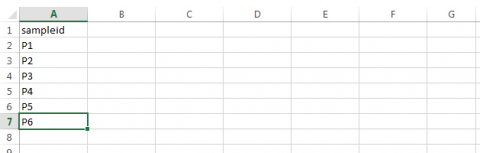
1. Assign a sampleid designator to the first column.

Step 2

With these parameters, we will use the Excel functions “IF” and “RAND” in the following steps:

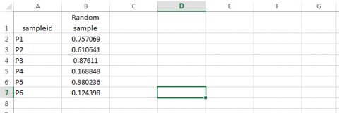
2. Obtain a random number from the Uniform Distribution for each of the sampleid’s. Syntax: type =RAND() in cell B2, then drag across all cells in column B.

Step 3

With these parameters, we will use the Excel functions “IF” and “RAND” in the following steps:

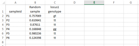
3. Based on the random number assigned to each sampleid, assign a genotype to the locus. Syntax: type =IF(B2<=0.09,”gg”,IF(B2>0.51,”tt”,”gt”)) in cell C1, then drag across all relevant cells. Note that values in columns B and C will likely differ from those in the example below.

Step 4

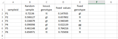
If we do not want the values generated by the RAND function to change as we add functions to the spreadsheet, we should plan to cut and paste a set of the actual values from one of the sampling events into new columns:

Other Population Structures

There are many other possible breeding population structures; some are the result of designed crosses (see Chapter 8 on mating designs), but most population structures emerge from long-term breeding programs in which elite homozygous cultivars are crossed to promising homozygous lines through opportunistic networks of crosses. Simulating genotypes at segregating loci from any mating design or breeding program can be obtained in a manner described in the previous paragraph. We need only decide on the frequencies of the genotypes in the segregating populations. For example, in the specific case of an F₂ generation derived from a cross of two inbred lines, p = q = 0.5, and if a random number obtained from a uniform distribution, U[0,1], is greater than ¼ and less than ¾ then the genotype of individual plant i, will be ‘gt’. We could be interested in the case of recombinant inbred lines derived in the F₅ generation of a cross of two inbred lines. In this case, the frequency of homozygotes is now p²+pqF and q²+pqF, and the frequency of heterozygous lines is 2pq(1-F), where F = 0.875. Thus, if a random number obtained from U[0,1] is less than 0.4687, then RIL. i will be assigned the genotype ‘gg’. It should be obvious that it should be possible to generate mixtures of segregating families from multiple independent or related crosses and simulate genotypes for any particular locus to all individuals in all families, regardless of how the families are derived.

Genetic Architecture of the Trait

Next, we need to decide how many loci will influence a trait and whether the alleles at the loci will interact. Let us begin with a single-locus additive quantitative trait, designated P. Further, consider a trait with an average phenotypic expression of 50 units and phenotypic variability in a diploid species that is due to additive genetic variability at a single locus and non-genetic variability. Initially, let us plan to let half of the phenotypic variability be due to segregation at the locus and half due to non-genetic sources of variability. The first step is to translate this brief description into a quantitative genetic model (Equation 1), preferably the same model that will be used in the eventual analysis of the phenotypic trait:

[latex]\large P_{ij} = \mu + G_i + \varepsilon_{ij}[/latex]

[latex]\textrm{Equation 1}[/latex] Quantitative genetic model for phenotypic trait,

where:
[latex]P_{ij}[/latex] = the phenotype,
[latex]G_i[/latex] = the genotype effect,
[latex]i[/latex] = one of three possible genotypes conferred by two alleles,
[latex]j[/latex] = one of the repeated samples of the i^th genotypes,
[latex]\varepsilon_{ij}[/latex] = non-genetic source of variability and is ~ i.id N(0,σ_ε).

Thus, the variance model of Equation 1 is as written in Equation 2:

[latex]\large \sigma^2_P = \sigma^2_G + \sigma^2_\varepsilon[/latex]

[latex]\textrm{Equation 2}[/latex] Variance model for phenotypic trait,

where:
[latex]\sigma^2_P[/latex] = the phenotypic variance,
[latex]\sigma^2_G[/latex] = the genotypic variance,
[latex]\sigma^2_\varepsilon[/latex] = residual or non-genotypic variance.

Parameter Assignment

The next step is to assign values to each of the parameters in the model. Mean, µ is assigned the value of 50, and values for e_ij are sampled from a Normal distribution with a mean of zero and a standard deviation of σ_e. We decided that we want to simulate data in which [latex]\large \sigma^2_P = \sigma^2_G + \sigma^2_\varepsilon[/latex] (Equation 2 above).

We can choose any value for σ²_P, but it is often best to choose a value that is ~ consistent with estimates from field trials for the crop of interest. In this case, let us say our field trials have typically produced estimates of phenotypic variance of ~ 98. Thus, both σ²_G and σ²_ε are ~ 49. Thus, we can obtain values for ε_ij by sampling a normal distribution with mean = 0 and standard deviation = 7.

Genotypic Values

We also need numeric values for each of the genotypes. Recall from Quantitative Genetic Models Theory we can assign coded genotypic values to each genotype as follows:

• Coded genotypic value of one homozygote (gg) = +a;
• Coded genotypic value of the other homozygote (tt) = -a;
• Coded genotypic value of heterozygotes (tg or gt) = d.

Since we are simulating an additive genetic model, the genotypic value of the heterozygotes (d) is midway between the two values for the homozygotes, i.e., d = 0. Thus,

G_i = a for i = “gg”; -a for i = “tt”; and 0 for i = “gt” or “tg”.

Now we need a numeric value for a.

Calculations

Recall that [latex]\sigma^2_P = \sigma^2_G + \sigma^2_\varepsilon[/latex] (Equation 2), and the additive portion of genetic variance is represented by Equation 3:

[latex]\sigma^2_A = 2pq[a +d(q-p)]^2,\;\;\;and\;\;\; \sigma^2_D = (2pqd)^2[/latex]

[latex]\textrm{Equation 3}[/latex] Formula for calculating additive genetic variance.

where:
[latex]\sigma^2_A[/latex] = the additive genetic variance,
[latex]\sigma^2_D[/latex] = the dominance variance,
[latex]\textrm{p and q}[/latex] = the frequency of the two alleles (g or t),
[latex]\textrm{a and d}[/latex] = coded genotypic values.

Since we have decided to simulate d = 0, the genetic variance is all due to additive effects ((Equation 4):

[latex]\sigma^2_G = \sigma^2_A = 2pqa^2[/latex]

[latex]\textrm{Equation 4}[/latex] Algebraic formula for calculating genotypic variance.

where:
[latex]\small \textrm{All terms}[/latex] are as defined previously.

Thus, [latex]a = \sqrt{\frac{49}{2pq}}.[/latex]

If we assume that the frequency of ‘t’ (or ‘g’) in the population is [latex]\frac{1}{4}[/latex], then a reasonable value for [latex]a = \sqrt{\frac{49}{2pq}} \tilde{} \small 19.80.[/latex]

Excel Application

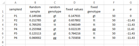
Next, let us translate these values for the parameters into Excel functions.

Syntax for assigning ‘a’: Type =IF(E3=“gg”,11.43, IF(E3=“tt”,-11.43,0)) in Cell G3, then drag across all relevant cells.

In order to fully understand how to sample from a normal distribution requires knowledge of probability density functions, cumulative density functions, and integral calculus that enables the translation between the two. These are topics beyond our current scope but worth exploring by those who wish to develop their own simulation capabilities.

Normal Distribution Interval

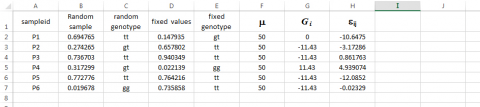
For our immediate purpose, the Syntax for obtaining values for ε_ij by sampling a Normal distribution with mean = 0 and standard deviation = 7 is the following:

Type =NORMINV(RAND(),0,7) in cell H3 and then drag across all relevant cells.

Simulated Phenotypes

We now have values for all of the parameters in the model and need merely sum columns F, G, and H to obtain the simulated phenotypes (column I) for each of the sampleids.

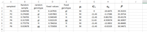
Keep in mind that if these were field trial data, we would only be able to obtain data found in columns A and I. It should be immediately apparent that column F could be a mean value for a particular replication or environment of the sampleids. Thus, it should be possible to simulate data from multiple replicates and multiple environments with different mean values. It should also be apparent that the sampling of ε_ij could be derived from environments with a different plot-to-plot variability. For example, instead of using 7 in the function =NORMINV(RAND(),0,7), we could designate the standard deviation for some environments to be 14 and thus create a type of GxE that we discussed in Chapter 12 on Multi Environment Trials.

Example Calculations

For the specific case of an F₂ generation derived from a cross of two inbred lines, p = q = 0.5, [latex]a = \sqrt{\frac{49}{2(0.25)}} = \small 9.9[/latex]

Alternatively, we could be interested in the case of recombinant inbred lines derived in the F₅ generation of a cross of two inbred lines. In this case,  the additive portion of genetic variance is represented by Equation 5:

[latex]\sigma^2_A = 2pq(1+F)[a+d(q-p)]^2[/latex]

[latex]\textrm{Equation 5}[/latex] Formula for calculating additive genetic variance involving inbreeding coefficient.

where:
[latex]\small F[/latex] = the coefficient of inbreeding,
[latex]\small \textrm{All terms}[/latex] are as defined previously.

Again, let d = 0, p = q = 0.5, but F = \small 0.875 and a reasonable value to simulate for [latex]a[/latex] as:

[latex]\large a = \sqrt{\frac{49}{2(1+F)pq}} \cong{} \small 7.23.[/latex]

Polygenic Trait Simulation

Let us next simulate a polygenic trait P in which segregation at three loci will contribute additive genotypic values that are responsible for 30% of the phenotypic variability. In this case, the phenotype is modeled where i, j, G, and ε are as before, and k represents each locus, while n is 3. For simplicity, let us assume that segregation at each of the three loci contributes an equal amount to the genotypic variability in an F₂ population. Let us refer to these loci as quantitative trait loci (QTL). Using the quantitative genetic models we have already used, we learn that for each of the simulated QTL, a can be obtained using Equation 6:

[latex]\large a = \frac{\large\sqrt{\frac{\sigma^2_G}{2pq}}}{\small nQTL},[/latex]

[latex]\textrm{Equation 6}[/latex] Formula for calculating additive genotypic value involving QTL,

where:
[latex]\small \textrm{All terms}[/latex] are as defined previously.

If we want the total phenotypic variability to be ~98, as before, and the frequency of each of the alleles at all three loci is 0.5 (as in an F₂), then σ²_G = σ²_A = 29 and a = 2.56 for each of the loci. We would translate this information to the Excel spreadsheet as before, but now the spreadsheet will have three columns for genotypes and three columns for genotypic values at each of the loci.

QTL Simulations

How would you simulate genotypic effects if you wanted one of the QTLs to contribute 75%, a second QTL to contribute 20%, and the third to contribute 5% to the total genotypic variability?

For hybrid crops, the segregating progeny are often evaluated in testcross combination. For example, in maize, it is routine to generate doubled haploids (DHs) from a cross of two elite Stiff Stalk homozygous lines. The DH’s are then crossed to an elite non-Stiff-Stalk homozygous ‘tester’. The resulting sample of Testcrossed DH (TDH) will be evaluated in an initial field trial. Let us simulate this situation for TDHs, grown in a field trial in which the CV for yield is ~ 7% and the mean is ~ 225 bu/ac. In order to simulate TDH’s we need to recall that the additive genetic variance for testcross progeny is represented by Equation 7:

[latex]\sigma^2_{A^T} = {1 \over 2}(1+F)(\alpha^T)[/latex]

[latex]\textrm{Equation 7}[/latex] Formula for calculating additive genetic variance for testcross progeny,

where:
[latex]\sigma^2_{A^T}[/latex] = the additive genetic variance for testcross,
[latex]F[/latex] = the coefficient of inbreeding,
[latex]\alpha^T[/latex] = the average effect of testcrossed allele.

Because the parents of the DH lines are fully homozygous, we can assume F=1. Thus, [latex]\sigma^2_{A^T} = \alpha^T[/latex].
Otherwise, the simulations will be generated as before, except we now have a different mean and phenotypic variance.

References

Beavis, W. D.1994. The power and deceit of QTL experiments: lessons from comparative QTL studies, p.250-266. In Proceedings of the forty-ninth annual corn and sorghum industry research conference. American Seed Trade Association, Washington, DC.

Bulmer, M. G. 1976. The effect of selection on genetic variability: a simulation study. Genet. Res., Camb. (1976), 28, pp. 101-117

Hill, W. G., and A. Robertson. 1968. Linkage disequilibrium in finite populations. Theor. Appl. Genet. 38, 226–231.

Podlich, D. W., and M. Cooper. 1998. Modelling plant breeding programs as search strategies on a complex response surface, p.171-178. In Asia-Pacific Conference on Simulated Evolution and Learning. Springer, Berlin, Heidelberg