
Chapter 1: Gene Frequencies
William Beavis; Kendall Lamkey; and Anthony Assibi Mahama
The challenge of Quantitative Genetics is to connect traits measured on quantitative scales with genes that are inherited and evaluated as discrete units. This challenge was addressed through the development of theory between 1918 and 1947. The theory is now referred to as the Modern Synthesis and required another 50 years for technological innovations and experimental biologists to validate. Luminaries such as RA Fisher, Sewell Wright, JBS Haldane, and John Maynard Smith were able to develop the theory that is still widely applied without the benefit of high throughput ‘omics’ technologies. Indeed, modern synthesis was developed before the knowledge of the structure of DNA.
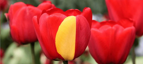
Population genetics characterizes how discrete units, i.e., alleles, change in breeding populations. Such characterization is the basis for understanding the structure of genomes and breeding populations. The forces of mutation (Fig. 1), migration, selection, and drift will alter the structure of breeding populations. Herein we will learn how to characterize population structure at one or two loci in diploid crop species. This will set the foundation for characterizing structure based on any number of loci and for polyploid crops that you may encounter in more advanced courses.
- Demonstrate the relevance of population genetics concepts to plant breeding populations.
- Demonstrate the relevance of a purely theoretical Ideal Population to plant breeding populations.
- Demonstrate understanding of the purpose of populations in Hardy-Weinberg Equilibrium
- Distinguish populations in Hardy-Weinberg Equilibrium from the Ideal Population.
- Describe the impact of mutation, selection, and drift on breeding populations.
Allelic and Genotypic Variation
Ideal Population
In order to understand the genetic structure of a population, it is necessary to establish a standard reference population so that the breeding population can be characterized relative to the standard. For this purpose, an ‘ideal’ conceptual base population can be defined as infinitely large with the potential to extract finite sub-populations through sampling, such as depicted in the following figure and described in Falconer and Mackay (1996):
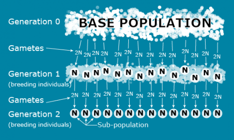
Note that the sub-populations depicted in Fig. 2 are based on a genetic sampling process that is affected by the reproductive biology of the species. Unlike animal species, crop species can reproduce in a variety of ways:
- Sexual
- Cross-Pollination
- Self-Pollination
- Mixtures of Self and Cross-pollination
- Asexual
- Clonal
- Doubled haploids
- Apomixis
Assumptions
In the ideal population depicted in Fig. 2, the following assumptions are true:
- The base population is infinite or at least too large to count.
- There is no migration between sub-populations.
- There is no breeding between overlapping generations.
- The number of breeding individuals is the same in each subpopulation.
- There is random mating within a subpopulation.
- There is no Selection.
- There is no Mutation.
Of course, in real populations, these assumptions are violated.
Allelic and Genotypic Frequencies
We first model a single locus with only two alleles in an ideal breeding population of diploid individuals. Define the following:
N = number of breeding individuals in a subpopulation (population size)
t = time usually measured in terms of generations
q = frequency of one of two alleles at a locus within a subpopulation
p = 1 – q = frequency of a second allele at a locus within a subpopulation
[latex]\overline{p}[/latex] = frequency of a second allele across the subpopulations (the mean of p)
p0 = frequency of a second allele in the base population
Due to the assumptions associated with an ideal reference population, [latex]\overline{q}[/latex] = q0 at any stage or generation of the sampling process, so q0 can be used interchangeably with [latex]\overline{q}[/latex].
The alleles, allele frequencies, genotypes, and genotypic frequencies can be represented in Table 1 and in Equations 1 and 2.
| Alleles | Genotypes | ||||
| A | a | AA | Aa | aa | |
| Frequencies | p | q | PAA | PAa | Paa |
[latex]p + q = 1[/latex].
[latex]\textrm {Equation 1}[/latex] Sum of allele frequencies.
[latex]P_{AA} + P_{Aa} + P_{aa} = 1[/latex].
[latex]\textrm {Equation 2}[/latex] Sum of genotype frequencies,
where:
[latex]p, q[/latex] are as defined earlier,
[latex]P_{AA}, P_{Aa}, P_{aa}[/latex] = frequencies of the three genotypes.
Variance of Allele Frequency
The relationship between allele frequencies and genotype frequencies can be expressed as in Equation 3.
[latex]p = P_{AA} + \frac{1}{2} P_{Aa}\;\; and\;\; q = P_{aa}+\frac{1}{2}P_{Aa}[/latex],
[latex]\textrm {Equation 3}[/latex] Equation for determining allele frequency,
where:
[latex]terms[/latex] are as defined earlier.
A particular sub-population is a random sample of N individuals or 2N gametes (for a diploid) from the base population. Therefore, the expected gene frequency of a particular allele in the sub-populations is q0, and the variance of q is represented by Equation 4.
[latex]\large \sigma_{q}^{2} = \frac{p_0q_0}{2N}[/latex].
[latex]\textrm {Equation 4}[/latex] Equation for estimating the variance of an allele,
where:
[latex]\sigma_{q}^{2}[/latex] = the variance of an allele,
[latex]N[/latex] = the number of individuals.
Since q0 is a constant, the variance of the change in allele frequency (q1 – q0) is also:
[latex]\large \sigma_{\Delta q}^{2} = \frac{p_0q_0}{2N}[/latex].
[latex]\textrm {Equation 5}[/latex] Equation for estimating the variance of change in allele frequency,
where:
[latex]\sigma_{\Delta q}^{2}[/latex] = the change in allele frequency,
[latex]\textrm{other terms}[/latex] are as defined before.
Frequency Estimators
In addition to the genetic sampling process depicted in Fig. 2, a statistical sampling process can be used to estimate frequencies, variances, and covariances of alleles and genotypes in a sub-population. If we sample n individuals from a population of size N, then notationally (Equation 6),
[latex]n = n_{AA} + n_{Aa} + n_{aa},\;\ \textrm{then}\;\ n_A = 2n_{AA} + n_{Aa}[/latex]
[latex]\textrm {Equation 6}[/latex] Equation for determining the number, n, of individuals and number of A individuals in a sample from a population,
where:
[latex]n[/latex] = the sample size,
[latex]\textrm{other terms}[/latex] are as defined before.
Estimates of the frequency of the [latex]A[/latex] allele and [latex]AA[/latex] genotype in the sample are obtained using Equation 7.
[latex]\hat{p}_A = \frac{1}{2n}n_A\;\ and\;\ \hat{p}_{AA}=\frac{1}{n}n_{AA}[/latex]
[latex]\textrm {Equation 7}[/latex] Estimating the frequency of A allele and AA genotype in a sample,
where:
[latex]\hat{p}_A[/latex] = the estimate of the A allele frequency,
[latex]\hat{p}_{AA}[/latex] = the estimate of the AA genotype frequency.
Expected Number of Alleles
Recognizing that statistical sampling at a locus with two alleles in a diploid population is represented as a binomial random process, the expected number of A alleles and their frequency in a sample can be determined using Equation 8.
[latex]E(n_A) = 2nP_{AA} + nP_{Aa}\;\ and\;\ E(\hat{p}_A) = P_A[/latex]
[latex]\textrm{Equation 8}[/latex] Estimating the expected number of a allele,
where:
[latex]E(n_A)[/latex] = the expectation of the A allele,
[latex]\textrm{Other terms}[/latex] are as defined previously.
Thus, [latex]\widehat{p}_A[/latex] is an unbiased estimator of the population parameter [latex]p_A[/latex].
Using the definition of variance, we can likewise find the [latex]Var(n_A)[/latex] and [latex]Var\left (\hat{p}_{A} \right)[/latex] using Equations 9 and 10. All terms have been defined previously.
[latex]Var(n_A) = 2n (p_A + P_{AA} - 2p_{A}^{2})[/latex]
[latex]\textrm{Equation 9}[/latex] Calculating the variance of n number of the A allele.
[latex]Var\left( \hat{p}_{A} \right)=\frac{1}{2n}\left ( p_{A} + P_{AA}-2p_{A}^{2} \right )[/latex]
[latex]\textrm{Equation 10}[/latex] Calculating the variance of the estimated frequency of the A allele.
Note that [latex]\text{}p_{A} \; \textrm{and} \; P_{AA}[/latex] are usually unknown, so we often substitute [latex]\text{}\hat{p}_{A} \; \textrm{and} \; \hat{P}_{AA}[/latex] in the calculation of the [latex]Var(\hat{p}_{A})[/latex]. Also, note that [latex]Var(\hat{p}_{A})[/latex] is not the variance of a Binomial distribution. If the population sampled is in Hardy-Weinberg Equilibrium (see below), the genetic sampling of alleles will be random so that [latex]P_{AA}=p_{A}^{2} \; \textrm{and} \; P_{Aa}=2p_{A}p_{a}[/latex]. The variance of the estimated frequency of the A allele can be obtained using Equation 11, which has the form of the variance from a binomial distribution.
[latex]Var\left ( \hat{p}_A \right )=\frac{1}{2n}p_{A}\left ( 1-p_{A} \right )[/latex]
[latex]\textrm{Equation 11}[/latex] Alternative equation for calculating the variance of estimated frequency of an allele.
where:
[latex]\textrm{terms}[/latex] are as defined previously.
Hardy-Weinberg Equilibrium
The proof of the Hardy Weinberg Equilibrium (HWE) requires the following assumptions (Falconer and Mackay, 1996):
- Allele frequency in the parents is equal to the allele frequency in the gametes.
-
- Assumes normal gene segregation.
-
- Assumes equal fertility of parents.
- Allele frequency in gametes is equal to the allele frequency in gametes forming zygotes.
- Assumes equal fertilizing capacity of gametes.
- Assumes a large population.
- Allele frequency in gametes forming zygotes is equal to allele frequencies in zygotes.
- Genotype frequency in zygotes is equal to genotype frequency in progeny.
- Assumes random mating.
- Assumes equal gene frequencies in male and female parents.
- Genotype frequencies in progeny do not alter gene frequencies in progeny.
- Assumes equal viability.
For a two-allele locus in a population in HWE, [latex]P_{AA} = p^2, P_{Aa} = 2pq, and\; P_{aa} = q^2[/latex].
HWE at a given genetic locus is achieved in one generation of random mating. Genotype frequencies in the progeny depend only on the allele frequencies in the parents and not on the genotype frequencies of the parents.
Disequilibrium
As discussed, there are several processes that can force allelic and genotypic frequencies to deviate from HWE. Deviations from equilibrium are referred to as disequilibrium and are often denoted with a disequilibrium coefficient, D. In the two allele case, the genotypic frequencies can be represented as [latex]P_{AA} = p_{A}^{2} + D_A, P_{Aa} = 2p_Ap_a - 2D_A, and\; P_{aa} = p_{a}^{2} + D_A[/latex].
Thus, the disequilibrium coefficient can be estimated using Equation 12.
[latex]\widehat{D}_A = \widehat{P}_{AA} - p_{A}^{2}[/latex].
[latex]\textrm{Equation 12}[/latex] Equation for estimating D.
where:
[latex]E(\widehat{D}_A)[/latex] = the estimate of the disequilibrium coefficient of the A allele,
[latex]\textrm{Other terms}[/latex] are as defined previously.
Note that the expectation of [latex]\widehat{D}_A[/latex] can be obtained from Equation 13. All terms are defined earlier.
[latex]E(\widehat{D}_A) = D_A - \frac{1}{2n}[p_A (1-p_A)+D_A][/latex].
[latex]\textrm{Equation 13}[/latex] Equation for estimating D.
The, [latex]\widehat{D}_A[/latex] is biased. Although the estimate of [latex]D_A[/latex] is biased, as the sample size, n, becomes large, the bias becomes small. Thus, emphasizing the need for large sample sizes in drawing inferences about disequilibrium from Hardy-Weinberg.
Variance
The [latex]Var(\widehat{D}_A)[/latex] can likewise be derived as (Equation 14:
[latex]\cong \frac{1}{n}[p_{A}^{2} (1 - p_A)^2 + (1 - 2p_A)^2 D_A - D_{A}^{2}][/latex].
[latex]\textrm{Equation 14}[/latex] Equation for estimating the variance of [latex]Var(\widehat{D}_A)[/latex].
If [latex]n[/latex] is large, [latex]E(\widehat{D}_A)\cong D_A[/latex], and [latex]\widehat{D}_A \sim N[E(\widehat{D}_A), Var (\widehat{D}_A)][/latex], a normal distribution.
So, a standard normal variate, [latex]Z[/latex] can be constructed as:
[latex]Z = \frac{\widehat{D}_A - E(\widehat{D}_A)} {\sqrt{Var (\widehat{D}_A)}}[/latex].
[latex]\textrm{Equation 15}[/latex] Equation for estimating the standard normal variate, Z.
Goodness of Fit
Alternatively, because [latex]Z^2 = \chi^2[/latex], therefore Equation 16 allows the calculation of chi-square.
[latex]\chi_{A}^{2} = \frac{nD_{A}^{2}}{p_{A}^{2}(1 - p_A)}[/latex],
[latex]\textrm{Equation 16}[/latex] Equation for estimating chi-square.
This form enables the direct use of genotypic counts, [latex]n_{AA}, n_{Aa}, n_{aa}[/latex], as shown in Table 2.
| n/a | Genotypes | ||
| n/a | AA | Aa | aa |
| Observed (O) | [latex]n{AA}[/latex] | [latex]n_{Aa}[/latex] | [latex]n_{aa}[/latex] |
| Expected (E) | [latex]np^2_A[/latex] | [latex]2p_{A}(1-p_{A})[/latex] | [latex]n(1-p_{A})^2[/latex] |
| O-E | [latex]n\hat D_{A}[/latex] | [latex]-2n\hat D_{A}[/latex] | [latex]n\hat D_{A}[/latex] |
The Goodness of Fit Statistic
Assessing the fit of observed data to expectation can be accomplished by using Equation 17.
[latex]\chi {_{A}^{2}} = \frac{(0-E)}{E}[/latex]
[latex]\textrm{Equation 17}[/latex] Formula for calculating chi-square goodness of fit statistic.
where:
[latex]O[/latex] = the observed data,
[latex]E[/latex] = expected data.
Non-Random Mating
Two methods of non-random mating that are important in plant breeding are assortative mating and disassortative mating.
Assortative mating occurs when similar phenotypes mate more frequently than they would by chance. One example would be the tendency to mate early x early maturing plants and late x late maturing plants. The effect of assortative mating is to increase the frequency of homozygotes and decrease the frequency of heterozygotes in a population relative to what would be expected in a randomly mating population. Assortative mating effectively divides the population into two or more groups where matings are more frequent within groups than between groups.
Disassortative mating occurs when unlike or dissimilar phenotypes mate more frequently than would be expected under random mating. Its consequences are, in general, opposite those of assortative mating in that disassortative mating leads to an excess of heterozygotes and a deficiency of homozygotes relative to random mating. Disassortative mating can also lead to the maintenance of rare alleles in a population.
Factors Affecting Allele Frequency
The factors affecting changes in allele frequency can be divided into two categories: systematic processes, which are predictable in both magnitude and direction, and dispersive processes, which are predictable in magnitude but not direction. The three systematic processes are migration, mutation, and selection. Dispersive processes are a result of sampling in small populations.
Migration
Assume a population has a frequency of m new immigrants each generation, with 1-m being the frequency of natives. Let qm be the frequency of a gene in the immigrant population and q0 the frequency of the same gene in the native population. Then the frequency in the mixed population will be:
[latex]q_1 = mq_m + (1 - m) q_0 = m(q_m - q_0) + q_0[/latex].
[latex]\textrm{Equation 18}[/latex] Formula for calculating the frequency of an allele in a mixed population.
where:
[latex]q_1[/latex] = the frequency of the allele,
[latex]\textrm{Other terms}[/latex] are as defined.
The change in gene frequency brought about by migration is the difference between the allele frequency before and after migration.
[latex]\Delta q = q_1 - q_0 = m (q_m - q_0)[/latex].
[latex]\textrm{Equation 19}[/latex] Formula for calculating the change in gene frequency.
Thus the change in gene frequency from migration is dependent on the rate of migration and the difference in allele frequency between the native and immigrant populations.
Mutations
Mutations are the source of all genetic variation. Loci with only one allelic variant in a breeding population have no effect on phenotypic variability. While all allelic variants originated from a mutational event, we tend to group mutational events into two classes: rare mutations and recurrent mutations, where the mutation occurs repeatedly.
Rare Mutations
By definition, a rare mutation only occurs very infrequently in a population. Therefore, the mutant allele is carried only in a heterozygous condition and, since mutations are usually recessive, will not have an observable phenotype. Rare mutations will usually be lost, although theory indicates rare mutations can increase in frequency if they have a selective advantage.
Fate of a Single Mutation
Consider a population of only AA individuals. Suppose that one A allele in the population mutates to a. Then there would only be one Aa individual in a population of AA individuals. So, the Aa individual must mate with an AA individual, i.e., [latex]AA \times Aa \to 1AA:1Aa[/latex]
This mating has the following outcomes Li (1976; pp 388):
- No offspring are produced, in which case the mutation is lost.
- One offspring is produced: the probability of that offspring being [latex]AA[/latex] is [latex]\frac{1}{2}[/latex], so the probability of losing the mutation is [latex]\frac{1}{2}[/latex].
- Two offspring are produced: [latex]Aa[/latex] can mate with more than one of the [latex]AA[/latex] individuals in the population, thus if [latex]Aa[/latex] mates with two [latex]AA[/latex] individuals, the probability of both offspring being AA is [latex]\frac{1}{4}[/latex], so the probability of losing the mutation is [latex]\frac{1}{4}[/latex].
If [latex]k[/latex] is the number of offspring from the above mating, then the probability of losing the mutation among the first generation of progeny is [latex](\frac{1}{2})^k[/latex].
Probability of Loss
The probability of losing the gene in the second generation can be calculated by making the following assumptions:
- The number of offspring per mating is distributed as a Poisson process (which means that they follow a stochastic distribution in which events occur continuously and independently of one another).
- With the average number of offspring per mating = 2.
- New mutations are selectively neutral.
With these assumptions, the probabilities of extinction are as in Table 3:
| Generation | Probability of Loss |
|---|---|
| 1 | 0.37 |
| 7 | 0.79 |
| 15 | 0.89 |
| 31 | 0.94 |
| 63 | 0.97 |
| 120 | 0.98 |
Recurrent Mutations
Let the mutation frequencies be:
[latex]\large{\text{Mutation Rate } \Large {\underset{p_o}{A} \overset{u} {\underset{v}\leftrightarrows} \underset{q_o}{a}}}[/latex]
Then the change in gene frequency in one generation at equilibrium is determined using Equation 20, where [latex]pu = qv[/latex], and [latex]q = \frac{u}{v+u}[/latex].
[latex]\Delta q = up_{0} - vq_{0}[/latex].
[latex]\textrm{Equation 20}[/latex] Formula for calculating the change in gene frequency due to mutation.
where:
[latex]u[/latex] = the rate of mutation of A to a allele,
[latex]v[/latex] = the rate of mutation of a to A allele
Other terms are as defined.
Conclusions
- Mutations alone produce very slow changes in allele frequency.
- Since reverse mutations are generally rare, the general absence of mutations in a population is due to selection.
Selection
Selection is one of the primary forces that will alter allele frequencies in populations. Selection is essentially the differential reproduction of genotypes. In population genetics, this concept is referred to as fitness and is measured by the reproductive contribution of an individual (or genotype) to the next generation. Individuals that have more progeny are more fit than those who have less progeny because they contribute more of their genes to the population.
The change in allele frequency following selection is more complicated than for mutation and migration because selection is based on phenotype. Thus, calculating the change in allele frequency from selection requires knowledge of genotypes and the degree of dominance with respect to fitness. Selection affects only the gene loci that affect the phenotype under selection—rather than all loci in the entire genome—but it also would affect any genes that are linked to the genes under selection.
Effects of Selection
Change in allele frequency: The strength of selection is expressed as a coefficient of selection, s, which is the proportionate reduction in gametic output of a genotype compared to a standard genotype, usually the most favored. Fitness (relative fitness) is the proportionate contribution of offspring.
Partial selection against a completely recessive allele: To see how the change in allele frequency following selection is calculated, consider the case of selection against a recessive allele:
| n/a | Genotypes | |||
| n/a | AA | Aa | aa | Total |
| Initial Frequencies | p2 | 2pq | q2 | 1 |
| Coefficient of Selection | 0 | 0 | s | n/a |
| Fitness | 1 | 1 | 1 – s | n/a |
| Gametic Contribution | p2 | 2pq | q2(1 – s) | 1 – sq2 |
Frequency Equations
The frequency of allele [latex]a[/latex] after selection is estimated using Equation 21:
[latex]q_1 = \large \frac{q^2(1-s)+ pq}{1-sq^2} = \frac{q-sq^2}{1 - sq^2}[/latex].
[latex]\textrm{Equation 21}[/latex] Formula for calculating the frequency of an allele following selection,
where:
[latex]s[/latex] = the selection differential (represented as a deviation from the population mean),
[latex]\small \textrm{Other terms}[/latex] are as defined.
The change in allele frequency is then represented as in Equation:
[latex]\Delta q = q_1 - q = \large \frac{q-sq^2}{1 - sq^2} - q = \large \frac{sq^2 (1 - q)}{1 - sq^2}[/latex].
[latex]\textrm{Equation 22}[/latex] Formula for calculating the change in allele frequency due to selection.
where:
[latex]\small \textrm{terms}[/latex] are as defined.
In general, you can show that the number of generations, [latex]t[/latex], required to reduce a recessive from a frequency of [latex]q_0[/latex] to a frequency of [latex]q_t[/latex], assuming complete elimination of the recessive, i.e., [latex]s = 1[/latex] is (Equation 23):
[latex]t = \frac{1}{q_t} - \frac{1}{q_0}[/latex]
[latex]\textrm{Equation 23}[/latex] Formula for calculating the number of generations required.
Small Population Size
Unlike the three systematic forces that are predictable in both amount and direction, changes due to small population size are predictable only in amount and are random in direction.
The effects of small population size can be understood from two different perspectives. It can be considered a sampling process, and it can be considered from the point of view of inbreeding. The inbreeding perspective is more interesting, but looking at it from a sampling perspective lets us understand how the process works.
Consequences of small population size
- Random genetic drift: random changes in allele frequency within a subpopulation
- Differentiation between subpopulations
- Uniformity within subpopulations
- Increased homozygosity
Example 1: Let q = 0.5 and N = 50, then
[latex]\sigma_{q}^{2} = \frac{(0.5)(0.5)}{100} = \small 0.0025\ , \textbf {and} \quad \sigma_q = 0.05[/latex]
Example 2: Let q = 0.5 and N = 4, then
[latex]\sigma_{q}^{2} = \frac{(0.5)(0.5)}{8} = \small 0.03125\ , \textbf {and} \quad\sigma_{q} = 0.1768[/latex]
Inbreeding and Small Populations
Inbreeding is the mating together of individuals that are related by ancestry. The degree of relationship among individuals in a population is determined by the size of the population. This can be seen by examining the number of ancestors that a single individual has:
| Generation | Ancestors |
|---|---|
| 0 | 1 |
| 1 | 2 |
| 2 | 4 |
| 3 | 8 |
| 4 | 16 |
| 5 | 32 |
| 6 | 64 |
| 10 | 1,024 |
| 50 | 1,125,899,906,842,620 |
| 100 | 1,267,650,600,228,230,000,000,000,000,000 |
| t | 2t |
Just 50 generations ago, note that a single individual would have more ancestors than the number of people that have existed or could exist on earth.
Therefore, in small populations, individuals are necessarily related to one another. Pairs mating at random in a small population are more closely related than pairs mating together in a large population. Small population size has the effect of forcing relatives to mate even under random mating; thus, with small population sizes inbreeding is inevitable.
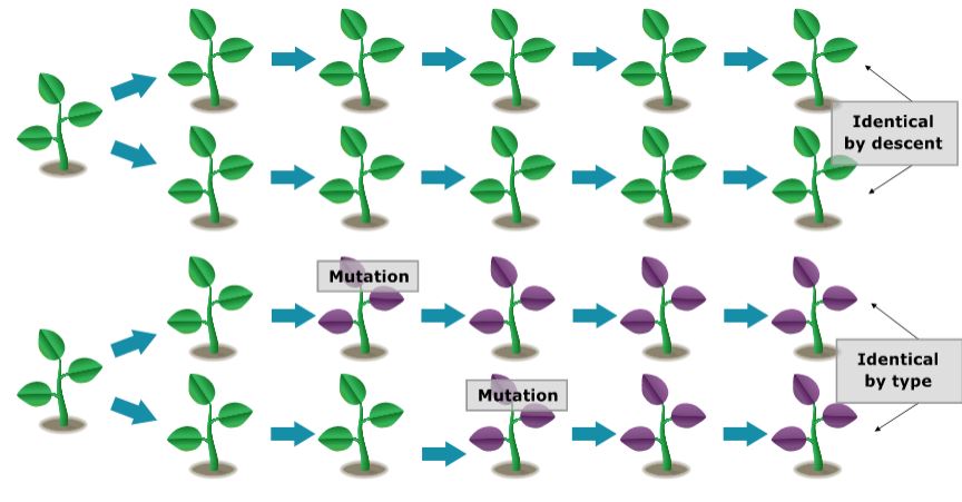
Identical by Descent and Identical by State
In finite populations, there are two sorts of homozygotes: Those that arose as a consequence of the replication of a single ancestral gene — these genes are said to be identical by descent (Bernardo, 1996). If the two genes have the same function but did not arise from the replication of a single ancestral gene, they are said to be alike in state. It is the production of homozygotes that are identical by descent that gives rise to inbreeding in a small population.
Coefficient of Inbreeding
The probability that two genes are identical by descent is called the coefficient of inbreeding and will be the measure of the relationship between mating pairs.
The coefficient of inbreeding (F) refers to the individual and expresses the degree of relationship between an individual’s parents. The coefficient of inbreeding is always expressed relative to a specified base population. The reference population is assumed to be non-inbred (F=0).
Consider a base population consisting of N individuals, each shedding equal numbers of gametes uniting at random. Because the base is non-inbred, each individual in this population carries genes that are non-identical. The only way a homozygote that carries genes that are identical by descent can arise is by the mating of a male and female gamete from the same individual that carries a replication of the same gene. Because there are 2N gametes, the probability that two mating gametes are identical by descent is [latex]\frac {1}{2N}[/latex].
Equation of Coefficient of Inbreeding
In the second generation, there are two ways genes are identical by descent can be joined:
- by a new replication of the same ancestral gene; and
- by the previous replication that occurred in generation 1.
The probability of a new replication event is [latex]\frac {1}{2N}[/latex]. The remaining proportion of zygotes, [latex]1 - \frac {1}{2N}[/latex], carry genes that are independent in origin from generation 1 but may have been identical in their origin in generation 0. The probability that the genes are identical by descent from generation 1 is the inbreeding coefficient of generation 1 is [latex]F_1 = \frac {1}{2N}[/latex].
Therefore, the probability of identical homozygotes in generation 2 is represent in Equation 23:
[latex]F_2 = \frac{1}{2N} + (1-\frac{1}{2N})F_{1}[/latex],
[latex]\textrm{Equation 23}[/latex] Formula for calculating the probability of identical homozygotes.
where:
[latex]\small F_1\ and\ F_2[/latex] = the inbreeding coefficients of generations 1 and progeny generation (PG),
[latex]\small N[/latex] = the population size.
The same arguments apply to future generations, so we can write the recurrence equation as (Equation 24):
[latex]F_t = \frac{1}{2N} + (1 - \frac{1}{2N})F_{t-1}[/latex].
[latex]\textrm{Equation 24}[/latex] Formula for calculating the probability of identical homozygotes in future generation.
where:
[latex]\small F_t[/latex] = the inbreeding coefficients of generation t,
[latex]\small N[/latex] = the population size.
Inbreeding Coefficient
The inbreeding of any generation is composed of two components: new inbreeding, which arises from self-fertilization, and the old, which was already there.
Note that inbreeding is cumulative and that the absence of inbreeding in generation [latex]t[/latex] does not change the fact that a population has inbreeding from prior generations.
Through a series of algebraic steps, we can write the inbreeding coefficient as a function of the number of generations removed from the reference populations (Equation 25):
[latex]F_1 = 1 - (1 - \Delta F)^t[/latex],
[latex]\textrm{Equation 25}[/latex] Formula for calculating the inbreeding coefficient.
where:
[latex]\small \Delta F = \frac{1}{2N}[/latex] is the change in inbreeding coefficients.
Dispersion
To relate inbreeding back to population size, we can rewrite the variance of the change in allele frequency [latex]\sigma^2_{\Delta q} = \frac{p_0q_0}{2N}[/latex] as (Equation 26):
[latex]\sigma^2_{\Delta q} = p_0q_0\Delta F[/latex],
[latex]\textrm{Equation 26}[/latex] Alternative formula for calculating the variance of the change in allele frequency.
And also represent the variance of the allele frequency as in Equation 27,
[latex]\sigma_{q}^{2} = p_0q_0F_t[/latex].
[latex]\textrm{Equation 27}[/latex] Alternative formula for calculating the variance of the allele frequency.
[latex]\Delta[/latex] expresses the rate of dispersion and [latex]F[/latex] expresses the amount of dispersion.
Changes in Frequencies
The genotype frequencies in a population can then be expressed as:
| n/a | n/a | n/a | Origin | |
| n/a | Original Frequencies | Change due to inbreeding | Independent | Identical |
| AA | [latex]p^2_0[/latex] | [latex]+ p_0q_0F[/latex] | [latex]=p^2_0(1-F)[/latex] | [latex]+p_0F[/latex] |
| Aa | [latex]2p_0q_0[/latex] | [latex]-2p_0q_0F[/latex] | [latex]=2p_0q_0(1-F)[/latex] | |
| Aa | [latex]q^2_0[/latex] | [latex]+p_0q_0F[/latex] | [latex]=q^2_0(1-F)[/latex] | [latex]+q_0F[/latex] |
The algebra summarizes what is expected to happen “asymptotically”. In any given breeding population, the results will vary due to sampling.
References
Bernardo, R. 1996. Best Linear Unbiased Prediction of Maize Single-Cross Performance Given Erroneous Inbred Relationships. Crop Sci. 36:862-866.
Falconer, D.S., and T.F.C. Mackay. 1996. Introduction to quantitative genetics. 4th ed. Pearson, Burnt Mill, England.
How to cite this chapter: Beavis, W., K. Lamkey, and A. A. Mahama. 2023. Gene Frequencies. In W. P. Suza, & K. R. Lamkey (Eds.), Quantitative Genetics for Plant Breeding. Iowa State University Digital Press.
Identification of individuals or lines that are more desirable than others in a heterogeneous population.
Relative ability of an individual to survive and reproduce to contribute its genes to the next generation.
