
Chapter 5: Gene Effects
William Beavis; Kendall Lamkey; Katherine Espinosa; and Anthony Assibi Mahama
In 1918, RA Fisher provided the first major contribution to the Modern Synthesis by proposing a model that reconciled the inheritance of discrete characteristics (Mendel) and continuous, or quantitative, characteristics (Darwin) in breeding populations. Herein, the same theoretical foundations are introduced.
For the beginning student, it will seem that the primary purpose of theory and modeling is to provide interpretations of observational and experimental results. Without this theoretical foundation, there would be no genetic understanding of the results from plant breeding experiments.
However, there is a more important practical justification for learning theoretical models: Theory provides predictions. Predictions are the basis for generating testable hypotheses. Also, with a theoretical model, it is possible to simulate many different breeding strategies. These can be compared, and the most promising can be used to design and implement the most effective and efficient breeding strategies. Thus, the theory provides a rational basis for designing plant breeding programs.
- Model Genotypic and Phenotypic Values of individuals in crop breeding populations.
- Integrate genotypic effect models with allele frequency models at single and multiple loci.
- Distinguish and estimate genetic effects, effects of allele substitutions, and Breeding Values at single and multiple loci.
- Distinguish and estimate dominance and epistatic deviations from additive effect models.
- Integrate concepts to applied breeding programs with data sets consisting of genotypic (marker) information with phenotypic information for QTL analyses.
Linear Models for Phenotypic Values
Single Locus
The phenotypic value of an individual, or group of individuals, is observed when a character or trait is measured. For example, if a corn plant was measured and found to be 275 cm tall, then that would be its phenotypic value for height.
To draw inferences about the genetic properties of a trait, we model phenotypic values using linear components. The most common model consists of a part due to genetics and a part due to non-genetic effects such as the environment. This is usually written as:
[latex]P = G + E[/latex],
[latex]\textrm{Equation 1}[/latex] Linear model for evaluating phenotype.
where:
[latex]P[/latex] is the phenotypic value,
[latex]G[/latex] is the genotypic value, and
[latex]E[/latex] represents the non-genetic factors.
If we assume that [latex]\small \sum E=0[/latex], then [latex]\small \sum P=\sum G[/latex], and [latex]\small \bar{P}=\bar{G}[/latex].
Population Mean
The mean phenotypic value of a population is equal to the mean genotypic value when the non-genetic (environmental) deviations sum to zero.
To calculate the expected genotypic properties of a population for a single locus, we assign arbitrary genotypic values to each locus.
Consider a single locus with two alleles [latex]A[/latex] and [latex]a[/latex].
Coded genotypic value of one homozygote [latex]AA[/latex] = [latex]+a[/latex].
Coded genotypic value of the other homozygote [latex]aa[/latex] = [latex]-a[/latex]
Coded genotypic value of a heterozygote [latex]Aa[/latex] = [latex]d[/latex].
We can arbitrarily designate the A allele as the allele that increases the genotypic value. The genotypic value of the heterozygotes (d) depends on the level of dominance:
Degree of Dominance
- No dominance when d = 0 (Fig. 1).

- If [latex]A[/latex] is dominant or partially dominant relative to the [latex]a[/latex] allele, then d is positive towards the AA genotype, as shown in Fig. 2.

- If a is dominant or partially dominant to the A allele, then d is negative (Fig. 3).

- If dominance is complete: d = +a or -a

- If there is overdominance: d is greater than +a or less than -a

Allele Frequencies and Population Mean (Table 1)
| n/a | Genotype | |||
| n/a | AA | Aa | aa | Total |
|---|---|---|---|---|
| Frequency | [latex]p^{2}[/latex] | [latex]2pq[/latex] | [latex]q^{2}[/latex] | 1 |
| Genotypic Value | [latex]Y_{AA}[/latex] | [latex]Y_{Aa}[/latex] | [latex]Y_{aa}[/latex] | n/a |
| Coded GV | [latex]+a[/latex] | [latex]d[/latex] | [latex]-a[/latex] | n/a |
| Freq. x Coded GV | [latex]+p^{2}a[/latex] | [latex]2pqd[/latex] | [latex]-q^{2}a[/latex] | [latex]=a(p-q) + 2pqd[/latex] |
| n/a | Genotype | n/a | ||
| n/a | AA | Aa | aa | Total |
| Frequency | [latex]0.64[/latex] | [latex]0.32[/latex] | [latex]0.04[/latex] | [latex]1[/latex] |
|---|---|---|---|---|
| Genotypic Value | [latex]16[/latex] | [latex]12[/latex] | [latex]0[/latex] | n/a |
| Coded GV | [latex]8[/latex] | [latex]4[/latex] | [latex]-8[/latex] | n/a |
| Freq. x Coded GV | [latex]5.8[/latex] | [latex]1.28[/latex] | [latex]-0.32[/latex] | [latex]14.08[/latex] |
Note: Coded Genotypic Values are obtained by subtracting the mid-parent value i.e., the midpoint between the genotypic values of the two homozygotes (Table 2).
Population mean [latex]=\bar{Y}=\mu+\;\textrm{Expected value of}\;g_{ij}[/latex], and [latex]mh=\textrm{mid-homozygote value}[/latex].
The population mean is estimated using Equation 2.
[latex]\bar{Y}= mh + a(p - q) + 2pqd[/latex].
[latex]\textrm{Equation 2}[/latex] Formula for calculating population mean.
where:
[latex]p[/latex] = frequency of A allele,
[latex]q[/latex] = frequency of a allele,
[latex]a[/latex] = coded genotypic values of AA, aa genotypes,
[latex]d[/latex] = coded genotypic value of Aa genotype.
Additive Gene Action
Applying Equation 2 and the data in Table 2, the population mean is calculated as shown below.
[latex]a = Y_{11} - [\frac{Y_{11}+Y_{22}}{2}][/latex]
[latex]a = 16 - [\frac{16+0}{2}][/latex]
[latex]d = Y_{12} - [\frac{Y_{12}+Y_{22}}{2}][/latex]
[latex]d = 12 - [\frac{16+0}{2}] = 4[/latex]
[latex]\bar{Y} = 8 + 0.64 \times 8 + 0.32 \times 4 + 0.04 \times (-8) = 14.08[/latex]
[latex]\bar{Y} = a(p - q) + 2pqd[/latex] is both the mean genotypic value and the mean phenotypic value of the population with respect to the trait.
Notice that if d = 0, the heterozygote genotype has no impact on the population mean, and we say that completely additive gene action exists.
Two Loci
Next, consider the contributions of alleles at more than one locus and find the joint effect on the mean (Table 3).
Consider two single loci:
- Genotypic value of [latex]\small AA[/latex] is [latex]a_A[/latex]
- Genotypic value of [latex]\small BB[/latex] is [latex]a_B[/latex]
Consider multiple loci:
- Genotypic value of [latex]\small AABB[/latex] is [latex]a_A + a_B[/latex].
- Total genotypic value is [latex]\small G_T[/latex] = [latex]\small G_A + G_B[/latex].
- The mid-homozygote genotypic value is the average of double homozygotes [latex]\small \;\textrm{(A1A1B1B1 and A2A2B2B2)}[/latex].
| Two-locus genotypic values and frequencies | A locus genotype | |||
|---|---|---|---|---|
| AA | Aa | aa | ||
| B locus genotype | Coded Genotypic Value/Freq. | [latex]\small{a_A}[/latex]
[latex]p^2_A[/latex] |
[latex]d_{A}[/latex]
[latex]\small {2p_A q_A}[/latex] |
[latex]\small{-a_A}[/latex]
[latex]q^2_A[/latex] |
| BB | [latex]\small{a_B}[/latex]
[latex]p^2_B[/latex] |
[latex]\small {G_T=μ+a_A+a_B}[/latex] [latex]p^2_Ap^2_B[/latex] |
[latex]\small {G_T=μ+d_A+a_B}[/latex] [latex]2p_Aq_Ap^2_B[/latex] |
[latex]\small {G_T = \mu +a_A+a_B}[/latex]
[latex]q^2_Ap^2_B[/latex] |
| Bb | [latex]d_{B}[/latex]
[latex]\small {2p_B q_B}[/latex] |
[latex]\small {G_T=μ+a_A+d_B}[/latex] [latex]p^2_A2p_Bq_B[/latex] |
[latex]\small{ G_T=μ+d_A+d_B}[/latex] [latex]2p_Aq_A(2p_Bq_B)[/latex] |
[latex]\small {G_T=μ+a_A+d_B}[/latex] [latex]q^2_A2p_Bq_B[/latex] |
| bb | [latex]-a_{B}[/latex]
[latex]q^2_B[/latex] |
[latex]\small{ G_T=μ+a_A-a_B}[/latex] [latex]p^2_Aq^2_B[/latex] |
[latex]\small{ G_T=μ+d_A-a_B}[/latex] [latex]2p_Aq_Aq^2_B[/latex] |
[latex]\small{ G_T=μ-a_A-a_B}[/latex] [latex]q^2_Aq^2_B[/latex] |
Population Mean
Population mean, [latex]\bar Y[/latex] = [latex]\mu[/latex] + Expected values of GA and GB
GA and GB are weighted averages based on allele frequencies and coded genotypic values. The population mean is then represented by Equation 3.
[latex]\bar{Y} = \mu + E(G_A + G_B) = E(G_A +G_B),\; or\; \bar{Y} = \mu + \{a_A(p_A-q_A) + 2p_Aq_Ad_A\} + \{a_B(p_B - q_B) + 2p_Bq_Bd_B\}[/latex]
[latex]\textrm{Equation 3}[/latex] Alternative formula for calculating population mean.
where:
[latex]G_A[/latex] = weighted average of A allele,
[latex]G_B[/latex] = weighted average of a allele,
[latex]E(G_A + G_B)[/latex] = expectation of sum of the two values,
[latex]\textrm{other terms}[/latex] are as defined previously.
A numerical example is given in Table 4.
| Two-locus genotypic values and frequencies | A locus genotype | |||
| AA | Aa | aa | ||
| B locus genotype | Boded Genotypic Value/Freq. | 8 0.64 |
4 0.32 |
-8 0.04 |
| BB | 4 0.04 |
12 0.0256 |
8 0.0128 |
-4 0.0016 |
| Bb | 2 0.32 |
10 0.2048 |
6 0.1024 |
-6 0.0128 |
| bb | -4 0.64 |
4 0.4096 |
0 0.2048 |
-12 0.0256 |
| Average at locus A | 6.24 | 2.24 | -9.76 | |
| Average at locus B | 10.08 | 8.08 | 2.08 | |
[latex]mh = \frac{12+(-12)+4+{-4}}{4}= 0[/latex]
[latex]\bar{Y} = \mu + E(G_A + G_B) = E(G_A +G_B) \\ \bar{Y} = \mu + \{a_A(p_A-q_A) + 2p_Aq_Ad_A\} + \{a_B(p_B - q_B) + 2p_Bq_Bd_B\} \\ \bar{Y} = 0 + \{8(0.8-0.2) + 2*0.8*0.2*4\} + \{4(0.2 - 0.8)+ 2*0.8*0.2*2\} \\ \bar{Y} = 0 + 6.08 -1.76 = 4.32[/latex]
Extension To More Than 2 Loci
We can extend the concept discussed above for two-locus case to more than two loci and calculate the population mean in a similar manner; where
- [latex]G_{T} = \sum G_{i}[/latex]
- midpoint is the average of the most extreme multi-locus-homozygotes
- Population mean = [latex]\bar{Y}[/latex], is represented by Equation 4
[latex]\bar{Y} = \mu + E(∑G_i) = \mu + ∑E(G_i)=\mu + ∑\{a_i(p_i - q_i) + 2p_iq_id_i\}=∑a_i(p_i - q_i) + 2∑p_iq_id_i[/latex]
[latex]\textrm{Equation 4}[/latex] Formula for calculating population mean involving more than two loci.
where:
[latex]E(∑G_i)[/latex] = expectation of the sum of all G values,
[latex]\textrm{other terms}[/latex] are as defined previously.
Average Genetic (Allelic) Effects
Individuals chosen as parents transmit only a sample consisting of ½ of its alleles. With selection, we are concerned with the transmission of value from parent to offspring. This cannot be determined based on genotypic value alone. Parents pass on their genes or alleles, NOT their genotypes, to the next generation. Genotypes are created anew in each generation. One result is that some aspects of the value of a particular genotype are unpredictable. Yet, selection theory can work only with the predictable aspects of the union of two gametes. Therefore, we introduce the average effect of a gene (allele) to represent this concept.
Key Concept: Although genotypes determine genotypic values, alleles and not genotypes are inherited by progeny.
Average effect of a gene (allele): The mean deviation from the population mean of individuals who received the gene (allele) from one parent is the average effect of the gene (allele). The effect of the other gene (allele) received from the remaining parent is represented as a random allele from the population … for this concept.
Formula of Average Effect of an Allele
Conceptually, let a number of gametes carrying the A allele unite at random with gametes from the population; then, the mean of the genotypes deviates from the population mean by an amount that is the average effect of the A gene. This represents the average allele effect and is the average deviation from the population mean of individuals who received a specific allele from one parent and the other allele at random from the population.
| Alleles | Genotypes, coded genotypic values and frequencies | Mean value of genotypes produced | Population mean to be deduced | Average effect of the allele ([latex]\alpha_{i}[/latex]) | ||
|---|---|---|---|---|---|---|
| n/a | [latex]AA[/latex] [latex]a[/latex] |
[latex]Aa[/latex] [latex]d[/latex] |
[latex]aa[/latex] [latex]-a[/latex] |
next gen | this gen | (next gen) — (this gen) |
| [latex]A[/latex] | [latex]p[/latex] | [latex]q[/latex] | [latex]pa + qd[/latex] | [latex][a(p - q) + 2dpq][/latex] | [latex]q[a + d(q - p)][/latex] | |
| [latex]a[/latex] | [latex]p[/latex] | [latex]q[/latex] | [latex]-qa + pd[/latex] | [latex][a(p - q) + 2dpq][/latex] | [latex]-p[a + d(q - p)][/latex] | |
The average effect of the A allele (or the α allele) from a single locus is designated as αA (or αa) and calculated for data presented in Table 5 as:
[latex]\alpha_{A}=q[a + d(q - p)] = 0.2[8 + (0.2 - 0.8)4]=1.12 \\ \alpha_{a}=-p[a +(q-p) d]=-0.8[8+(0.2-0.8)4]=-4.48[/latex]
Allele Substitution Effect
The average effect of an allele substitution, often designated as  , is the difference between the average effects of each allele (Equation 5).
[latex]\alpha=\alpha_{A}-\alpha_{a}=a + d(q - p)[/latex]
[latex]\textrm{Equation 5}[/latex] Formula for calculating the average effect of allele substitution.
where:
[latex]\alpha_{A}, \alpha_{a}[/latex] = the average effects of allele A and a, respectively,
[latex]\textrm{other terms}[/latex] are as defined previously.
For example, from Table 5, [latex]\alpha_{1}[/latex] and [latex]\alpha_{2}[/latex] represent average allele effects of [latex]A[/latex] and [latex]a[/latex], respectively.
Average effects of each allele can be calculated as:
[latex]\alpha_{A}=q\alpha =0.2(5.6)=1.12 \\ \alpha_{a}=-p\alpha =(-0.8)( 5.6 )=-4.48[/latex]
Thus, the average effect of allele substitution =
[latex]\alpha=\alpha _{A}-\alpha _{a}=1.12-(-4.48)=5.6[/latex]
Note the average genetic effect is:
- Dependent on genotypic value,
- Dependent on gene frequencies,
- A property of the population as well as the genes concerned.
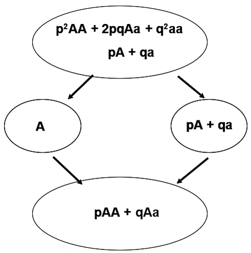
Breeding Value
Breeding value is a concept that is based on the following:
- The average value of a parent is judged by its progeny.
- Alleles carried by an individual and transmitted to its offspring can be inferred from the progeny,
- Which represents the sum of the average effects of all alleles an individual carries.
Let us use the average effect of alleles to rewrite the Equation 1 as:
[latex]P = G + E = \alpha _{i}+\alpha _{j}+\delta _{\ddot{y}}+E[/latex]
[latex]\textrm{Equation 6}[/latex] Alternative formula for calculating phenotypic value based on average effect of alleles.
where:
[latex]\alpha_{i}, \alpha_{j}[/latex] = the average effects of allele i, j in a diploid individual i, j, respectively,
[latex]\delta_{\ddot{y}}[/latex] is the dominance deviation.
Breeding value is the value of an individual judged by the average value of its progeny. The breeding value of an individual is equal to the sum of the average effects of the alleles it carries. The summation is over pairs of alleles at a locus and over all loci (Table 5). It is defined as twice the expected deviation of the individual’s progeny mean from the population mean when the individual is mated at random to other individuals from the same population (Tables 6 and 7).
Mean Breeding Value in Random Population
The mean breeding value in a random mating population is zero.
| Genotype | Breeding value |
|---|---|
| [latex]AA[/latex] | [latex]2\alpha_{A}=2q\alpha[/latex] |
| [latex]Aa[/latex] | [latex]\alpha_{A}+\alpha_{a}=(q-p)\alpha[/latex] |
| [latex]aa[/latex] | [latex]2\alpha_{a}=-2q\alpha[/latex] |
| Genotype | Breeding value |
|---|---|
| [latex]AA[/latex] | [latex]2\alpha_{A}=2(0.2)(5.6)=2.24[/latex] |
| [latex]Aa[/latex] | [latex]\alpha_{A}+\alpha_{a} =(0.2 - 0.8) 5.6=-3.36[/latex] |
| [latex]aa[/latex] | [latex]2\alpha_{a}=-2(0.8)(5.6)=-8.96[/latex] |
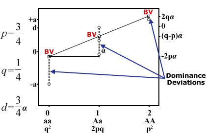
Deviations for Average Genetic Effects
Dominance Deviation
For a single locus: the difference between the genotypic value and the breeding value of a particular genotype is known as the dominance deviation. It is associated with the [latex]Aa[/latex] genotype. [latex]\delta_{ij}[/latex] represents the deviation of genotypic value (i.e., [latex]G_{ij}[/latex]) from the regression-fitted genotypic value and is zero when dominance is absent ([latex]d = 0[/latex])
Consider Genotype [latex]AA[/latex]. Recall that the Coded genotypic value of [latex]AA[/latex] = [latex]+a[/latex], and the population mean equals [latex]=a(p-q)+2dpq[/latex].
If a is expressed as deviation relative to the population mean, then is can be calculated using Equation 7.
[latex]a-\left[ a(p-q)+2dpq \right]=a(1-p+q)-2dpq=2qa-2dpq=2q(a-dp)[/latex]
[latex]\textrm{Equation 7}[/latex] Alternative formula for calculating average effect of allele substitution.
where:
[latex]a[/latex] = the average effect of allele substitution,
[latex]\textrm{other terms}[/latex] are as defined previously.
Notice that if d is not 0, and p is not equal to q, then a is affected by d. Also, recall that a can be expressed in terms of the average effect of an allele substitution (Equations 8 and 9), where terms are as defined previously,
[latex]a=\alpha-d(q-p)[/latex]
[latex]\textrm{Equation 8}[/latex] Alternative formula for calculating average effect of allele substitution.
Thus
[latex]2q(a-dp)=2q(\alpha-d(q-p)-dp)=2q(\alpha-dq+dp-dp)=2q(\alpha-dp)[/latex]
[latex]\textrm{Equation 9}[/latex] Alternative formula for calculating average effect of allele substitution.
Using similar algebra, the dominance deviation is represented by Equation 10 as,
[latex]\delta_{ij}=2q(\alpha-dp)-2pq=-2q^2d)[/latex]
[latex]\textrm{Equation 10}[/latex] Alternative formula for calculating the dominance deviation.
Observations About Dominance
Notice that
- If there is no dominance, d is zero, and the dominance deviations are also zero.
- In the absence of dominance, breeding values and genotypic values are the same.
- Alleles involved with genotypes that show no dominance, i.e., d = 0, are sometimes called ‘additive genes’, or are said to ‘act additively’.
Breeding Values and Dominance Deviations
As shown in Equation 6 the algebra of breeding values and dominance deviations provides the theoretical basis for subdividing the G component of the Phenotypic model,
[latex]P = G + E = \alpha _{i}+\alpha _{j}+\delta _{\ddot{y}}+E[/latex]
Thus, based on the algebra and substituting data from Table 7, dominance deviation is calculated as shwon below.
[latex]{\delta _{AA} =G_{AA}-\mu -\alpha _{A}-\alpha _{A}} =a-\mu -2(pa+qd-\mu) =-2q^{2}d[/latex]
[latex]=-2(0.2)2(4)=-0.32[/latex]
[latex]{\delta _{Aa} =G_{Aa}-\mu -\alpha _{A}-\alpha _{a}}=d-\mu -( pa + qd-\mu )-( pd-qa-\mu )=2pqd[/latex]
[latex]=2( 0.8) ( 0.2 ) ( 4 )=1.28[/latex]
[latex]{\delta _{aa}=G_{aa}-\mu -\alpha a}=-a-\mu -2( pd-qa-\mu)=-2p^{2}d[/latex]
[latex]=-2(0.8^2) (4)=-5.12[/latex]
Epistasis
Epistasis exists when genotypes at two or more loci result in a genotypic value that is greater or less than the sum of the average genotypic effects at each of the individual loci. For example,
| Genotype at Locus A | Genotype at Locus B | ||
|---|---|---|---|
| n/a | BB | Bb | bb |
| AA | 22 | 18 | 6 |
| Aa | 20 | 16 | 4 |
| aa | 14 | 10 | -2 |
| Genotype at Locus A | Genotype at Locus B | ||
|---|---|---|---|
| n/a | BB | Bb | bb |
| AA | 24 | 18 | 6 |
| Aa | 20 | 16 | 4 |
| aa | 14 | 10 | -2 |
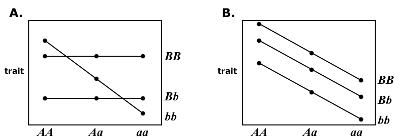
Graphical View of Epistasis
Epistasis between loci within an individual can be represented as the reaction norm of different genotypes at one locus, plotted against the genotypes at a second locus.
Figure 8A: Epistasis between loci occurs because the reaction norms of the locus B genotypes differ in slope.
Figure 8B: The reaction norms are parallel; thus, the effects of the two loci are independent, and no epistasis is present.
Physiological and Statistical Dominance
Cheverud and Routman (1995) identified two concepts associated with the term epistasis: physiological epistasis and statistical epistasis.
The distinction between these two concepts is similar to that made between physiological and statistical dominance:
Physiological Dominance:
- Heterozygote is not midway between two homozygotes.
- Values of a and d are not dependent on allele frequencies.
- When d ≠ 0, it reflects intralocus interaction is present.
- Least-squares solution of the unweighted regression of the number of genotypic values on the number of “a” alleles.
- Physiological dominance contributes to both additive and dominance values and variances.
Statistical Dominance Deviations:
- Deviations of single-locus from the additive combination of alleles contribute to the genotype.
- Depend on allele frequencies and will change with changes in allele frequencies.
- Least-squares solution of a weighted (weighted by genotypic frequencies) regression of genotypic value on the number of alleles.
Physiological Epistasis
In physiological epistasis (or mechanistic epistasis):
- Interaction effects occur “within” genotypes, where genes expressed within a single genome interact.
- Simply recognizes that certain genotypes at two or more loci interact in the production of a phenotype.
- If all possible genotypic classes are equally frequent in a population, the influence of genetic interactions on phenotypes will be directly observable.
- The contribution of physiological epistasis to populations is a function of the frequencies of interacting genotypes in a population.
Model for Physiological Epistasis
Let the phenotypic value of an individual be determined by the combination of the alleles present at two loci. This model is used to illustrate how physiologically based gene interactions map to components of genetic variation.
Consider the two loci, each with two alleles per locus; the two-locus (physiological) genotypic values, Gijkl, are the average phenotype of individuals with the ijth genotype at the first locus, and the klth genotype at the second locus. Notice that we are not given the genotypic values for the A locus nor for the B locus. So, we will determine the unweighted marginal means for each genotype.
| n/a | [latex]AA[/latex] | [latex]Aa[/latex] | [latex]aa[/latex] | Unweighted marginal mean |
|---|---|---|---|---|
| [latex]BB[/latex] | [latex]G_{AABB}=22[/latex] | [latex]G_{AaBB}=18[/latex] | [latex]G_{aaBB}=6[/latex] | [latex]G_{..BB}=15.33[/latex] |
| [latex]Bb[/latex] | [latex]G_{AABb}=20[/latex] | [latex]G_{AaBb}=16[/latex] | [latex]G_{aaBb}=4[/latex] | [latex]G_{..Bb}=13.33[/latex] |
| [latex]bb[/latex] | [latex]G_{AAbb}=14[/latex] | [latex]G_{Aabb}=10[/latex] | [latex]G_{aabb}=-2[/latex] | [latex]G_{..bb}=7.33[/latex] |
| Unweighted marginal means | [latex]G_{AA..}=18.66[/latex] | [latex]G_{Aa..}=14.66[/latex] | [latex]G_{aa..}=2.66[/latex] | [latex]G_{....}=12[/latex] |
Single Locus Genotype
The single-locus genotype is defined as the unweighted average across the genotypes at the second locus, for example, Equation 11.
[latex]G_{ij..} = \frac{(G_{ij11} + G_{ij12} +G_{ij22})}{3}, \; G_{..kl} = \frac{(G_{11kl} + G_{12kl} + G_{22kl})}{3}[/latex]
[latex]\textrm{Equation 11}[/latex] Alternative formula for calculating the dominance deviation.
where:
[latex]G_{ij..}, G_{..kl}[/latex] = the single locus genotype value.
Thus, the value at locus A is,
[latex]G_{AA..} = \frac{(22+20+14)}{3} = 18.66[/latex]
and at locus B is,
[latex]G_{..BB} = \frac{(22+18+6)}{3} = 15.33[/latex]
Non-Epistatic Genotypic Value
Subscripts [latex]A[/latex] and [latex]a[/latex] or [latex]B[/latex] and [latex]b[/latex] refer to the two alleles at the interacting loci. The single locus values of [latex]a[/latex] and [latex]d[/latex] are computed as in Equation 12.
[latex]a_{i}=G_{11..}-\frac{(G_{11..}+G_{22..})}{2}, \; d_{i}=G_{12..}-\frac{(G_{11..}+G_{22..})}{2}[/latex]
[latex]\textrm{Equation 12}[/latex] Formula for calculating the single locus values,
where:
[latex]a_{i}, d_{i}[/latex] = the single locus values.
Thus, the value at locus A is,
[latex]a_{A}=G_{11..}-\frac{(G_{11..}+G_{22..})}{2}=18.66-\frac{18.66+2.66}{2}=18.66-10.66=8[/latex]
and
[latex]d_{A}=G_{12..}-\frac{(G_{11..}+G_{22..})}{2}=14.66-\frac{18.66+2.66}{2}=14.66-10.66=4[/latex]
Similarly, [latex]a_{A}[/latex] and [latex]d_{A}[/latex] can be calculated to be 4 and 2, respectively. Try it!
The non-epistatic genotypic value, [latex]ne_{ijkl}[/latex], is calculated using Equation 13, represented by,
[latex]ne_{ijkl}=G_{ij..}+G_{..kl}-G_{....}[/latex]
[latex]\textrm{Equation 13}[/latex] Formula for calculating the non-epistatic genotypic value,
where:
[latex]\textrm{all terms}[/latex] are as defined previously.
For AABB genotype,
[latex]ne_{AABB}=G_{AA..}+G_{..BB}-G_{....}=18.66+15.33-12=21.99[/latex].
Epistatic Genotypic Value
| n/a | [latex]AA[/latex] | [latex]Aa[/latex] | [latex]aa[/latex] |
|---|---|---|---|
| [latex]BB[/latex] | [latex]21.99[/latex] | [latex]17.99[/latex] | [latex]5.99[/latex] |
| [latex]Bb[/latex] | [latex]19.99[/latex] | [latex]15.99[/latex] | [latex]3.99[/latex] |
| [latex]bb[/latex] | [latex]13.99[/latex] | [latex]9.99[/latex] | [latex]-2.01[/latex] |
The epistatic genotypic value is represented by Equation 14.
[latex]e_{ijkl} = G_{ijkl} - ne_{ijkl}[/latex]
[latex]\textrm{Equation 14}[/latex] Formula for calculating the epistatic genotypic value.
Example from data in Table 11 is,
[latex]e_{ijkl} = 22 - 21.99 = 0.01.[/latex]
A value of [latex]e_{ijkl}[/latex] different from zero indicates that Physiological Epistasis is present. In this example, there is little evidence for epistasis for this cell. Is there evidence for epistasis in the other cells?
Statistical Epistasis
In statistical epistasis (or population epistasis):
- The term is used to refer to the amount of population variation in genotypic values associated with variation among loci.
- Notation that is often used includes [latex]V_i[/latex], or [latex]G_{AxB}[/latex], or [latex]I_{AxB}[/latex].
- The amount of statistical epistasis present in a population is a function of the frequencies of interacting multilocus genotypes and therefore is a function of population allele frequencies as it is for additive and dominance variance ([latex]V_{A}\;\textrm{and}\;V_{D}[/latex]). It is calculated using Equation 15.
[latex]G_{T}=G_{A}+G_{B}+G_{A\times B}[/latex]
[latex]\textrm{Equation 15}[/latex] Formula for calculating the statistical genotypic value.
where:
[latex]G_{T}[/latex] = the total epistatic (statistical) value,
[latex]G_{A}[/latex] = value at locus A,
[latex]G_{B}[/latex] = value at locus B,
[latex]G_{B}+G_{A\times B}[/latex] = value due to A by B interaction.
Presence of epistasis between locus [latex]A[/latex] and [latex]B[/latex] changes the population mean, ([latex]Y[/latex]), mid-homozygote value ([latex]\mu[/latex]), [latex]a[/latex] (additive), and [latex]d[/latex] (dominance) values.
| Two-locus genotypic values and frequencies | A locus genotype | |||
| AA | Aa | aa | ||
| B locus genotype | Coded Genotypic Value/Freq | [latex]8[/latex] [latex]0.64[/latex] |
[latex]4[/latex] [latex]0.32[/latex] |
[latex]-8[/latex] [latex]0.04[/latex] |
| BB | [latex]4[/latex] [latex]0.04[/latex] |
[latex]24[/latex] [latex]0.0256[/latex] |
[latex]18[/latex] [latex]0.0128[/latex] |
[latex]6[/latex] [latex]0.0016[/latex] |
| Bb | [latex]2[/latex] [latex]0.32[/latex] |
[latex]20[/latex] [latex]0.2048[/latex] |
[latex]16[/latex] [latex]0.1024[/latex] |
[latex]4[/latex] [latex]0.0128[/latex] |
| bb | [latex]-4[/latex] [latex]0.64[/latex] |
[latex]14[/latex] [latex]0.4096[/latex] |
[latex]10[/latex] [latex]0.2048[/latex] |
[latex]-2[/latex] [latex]0.0256[/latex] |
| Average at locus A | [latex]16.32[/latex] | [latex]12.24[/latex] | [latex]0.24[/latex] | |
| Average at locus B | [latex]21.36[/latex] | [latex]18.08[/latex] | [latex]12.08[/latex] | |
Epistasis Effects
The genotypic value of AABB has been increased from 22 to 24 due to epistatic effects.
There are changes in population mean, mid-homozygote values for A and B locus, and the average at A and B locus as shown in calculations below.
[latex]\textrm{Epistatic effects between}\; AABB=2 \\ \eqalign {G_{T} &=\mu +G_{A}+G_{B}=10+8+4=22 \\ \textrm{With epistatic effects} \; G_{T} &=\mu +G_{A}+G_{B}+G_{A\times B}=10+8+4+2=24 }[/latex]
[latex]\textrm{Changes in the mid-homozygote}\; (\mu)=\frac {24+(-2)}{2}=11[/latex]
[latex]\eqalign {\textrm{Changes in the mean population}\;(Y)=14.37 \\ \mu _{A}=8.28 \\ \mu _{B}=16.72 \\ G_{A}: +a=8.04;d=3.96;-a=-8.04 \\ G_{B}: +a=4.64;d=1.36;-a=-4.64 }[/latex]
References
Cheverud, J. M. and E. J. Routman. 1995. Epistasis and its contribution to genetic variance components. Genetics, 139, 1455±1461.
How to cite this chapter: Beavis, W., K. Lamkey, K. Espinosa, and A. A. Mahama. 2023. Gene Effects. In W. P. Suza, & K. R. Lamkey (Eds.), Quantitative Genetics for Plant Breeding. Iowa State University Digital Press.
