
Chapter 10: G x E
William Beavis; Kendall Lamkey; Katherine Espinosa; and Anthony Assibi Mahama
One of the most difficult aspects of plant breeding involves making decisions about environments to target for the development of new cultivars. This challenge is not especially difficult if cultivars are adapted to large geographic regions with little variability among environments or if there is significant variability among environments, but potential cultivars respond similarly to the environmental differences. However, if potential cultivars do not respond similarly to environmental differences within a targeted set of environments, i.e., there are genotype-by-environment interactions, decisions on which genotypes to develop can be difficult. Herein, we explore the impacts of environments on genotypes in cultivar development programs.
- Conceptual types of GxE interactions.
- Decompose GxE interactions into heterogeneous variability and inconsistent rankings.
- Leverage information on heterogeneous variance and inconsistent rankings to meet breeding objectives.
Environmental Components of Variance
Recall that our working model for the phenotype includes genotypic and non-genotypic (environmental) sources of variability (Equation 1):
[latex]P=\mu+G+E[/latex]
[latex]\textrm{Equation 1}[/latex] Linear model for sources of variability in phenotype.
where:
[latex]P[/latex] = phenoype,
[latex]\mu[/latex] = overall mean,
[latex]G[/latex] = genotype effects ,
[latex]E[/latex] = non-genetic of environment effects.
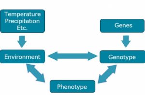
Briefly, we consider the components of E as shown in Fig. 1.
Many Meanings of Environment
Micro-environmental effects: the environment of a single organism as opposed to that of another growing at the same time and in almost the same place.
- All things except genotype affect a plant’s development. Note that the probability that two plants in the same field will experience the same environment is infinitesimally small.
- Physical and chemical properties of the soil
- Climatic variables (rain, temperature, etc)
- Solar radiation
- Biotic stresses
Macro-environmental effects: the general environment associated with a field site over a period of time.
- Different class of environments in one area or time than another
- A collection of micro-environments
Environmental Sources of Variation
Environmental sources of variation can also be hierarchically modeled to consist of variability among environments and within environments (Equation 2):
[latex]\sigma^2_E = \sigma^2_{among} + \sigma^2_{within}[/latex]
[latex]\textrm{Equation 2}[/latex] Formula for among and within sources of variability.
where:
[latex]\sigma^2_E[/latex] = environmental variance,
[latex]\sigma^2_{among}[/latex] = among environment variance,
[latex]\sigma^2_{within}[/latex] = within environment variance.
[latex]P_{ij}=\mu + G_{i} + E_{j}[/latex]
[latex]\textrm{Equation 3}[/latex] Model for phenotypic response.
where:
[latex]P_{ij}[/latex] = phenotype,
[latex]\mu[/latex] = overall mean,
[latex]G_{i}[/latex] = genotype effect,
[latex]E_{j}[/latex] = environment effect.
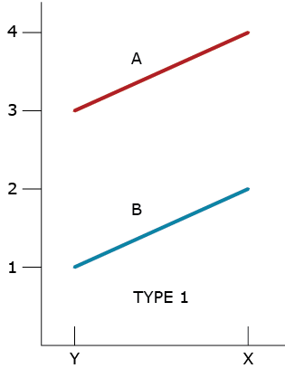
From the beginning of field assessments of clonally propagated plants, we have been able to recognize variability within and among locations (environments). As soon as we could evaluate more than one replicated genotype, we also began to recognize patterns of phenotypic responses to environments. In 1964, Allard and Bradshaw provided a simple classification scheme of the types of phenotypic responses that could happen using two genotypes (designated A and B) and two environments (designated X and Y) and modeled as in Equation 3. The first type of response (Type 1) reveals that there is a difference of 2 units between the genotypes and a difference of 1 unit between the environments (Fig. 2). They also recognized a second type of response (Type 2) in which the difference between genotypes was one unit while the difference between environments was 2 units. Both types of responses indicate no interaction.
Simple Types of GxE Interactions
These types of interaction can all be modeled as (Equation 4):
[latex]P_{ij}=\mu + G_{i} + E_{j} + GE_{ij}[/latex]
[latex]\textrm{Equation 4}[/latex] Model for phenotype response with GxE present.
where:
[latex]P_{ij}[/latex] = phenotypic response,
[latex]\mu[/latex] = overall mean,
[latex]G_{i}[/latex] = genotype effects,
[latex]E_{j}[/latex] = environment effects,
[latex]GE_{ij}[/latex] = genotype by environment interaction effect.
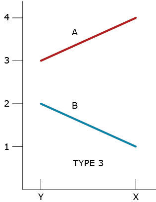
Type 3 GxE Interaction
Allard and Bradshaw recognized that there could be a lack of consistent responses by two different genotypes in two environments. The lack of consistent responses by genotypes to different environments had been recognized as genotype by environment interactions since the beginning of replicated trials, and Allard and Bradshaw classified these into four types of GxE for two genotypes in two environments.
A type 3 GxE response (Fig. 3) was based on the heterogeneity of genotypic variability between environments. Assuming that larger phenotypic values are desired, in GxE types 1,2, and 3, genotype A is better adapted to both types of environments.
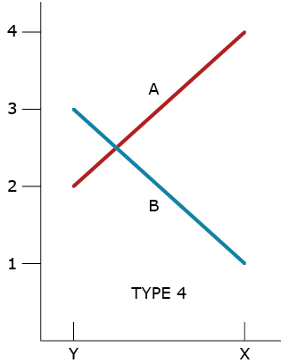
Type 4 GxE Interaction
A type 4 GxE interaction is due to a combination of heterogeneous genotypic variability and a failure of the genotypes to have correlated responses (change of rank) across the environments (Fig. 4).
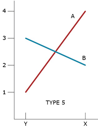
Type 5 GxE Interaction
A type 5 GxE is due to a failure of the genotypes to have correlated responses across the environments, while the genotypic variability is homogeneous between the environments (Fig. 5). If environments X and Y represent typical types of environments in a market, then there are unique best genotypes for each type of environment; neither is broadly adapted to both environments.
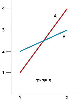
Type 6 GxE Interaction
A type 6 GxE interaction illustrates a ‘racehorse’ response by Genotype A. It takes full advantage of favorable environment X while failing under the stressful environment Y. This type of GxE also illustrates a more ‘stable’ response by Genotype B. The question for the plant breeder is whether to develop both types of cultivars or just one.
Complex Types of GxE Interactions
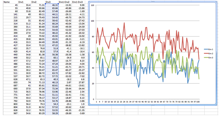
As the number of environments and genotypes increases, the ability to sort out the types of GxE interactions becomes more difficult. For example, consider the data and plot in Fig. 7. It is likely that all types of GxE interactions are present in these data. If all types of GxE are present, are there prevalent types of GxE? Do the genotypes behave the same way in some pairs of environments? What is the nature of GxE between all pairs of environments (1:2, 1:3, 2:3 …)?
To answer these questions, multi-variate statistical techniques, sometimes referred to as pattern analyses, are used to discover and summarize consistent patterns in large data sets.
Pattern Analysis Methods
A partial listing of these pattern analysis methods would include Cluster Analyses (CA), Principal Component Analysis (PCA), Additive Main and Multiplicative Interaction (AMMI) models, Sites Regression models, Partial Least Squares, Factorial Regression, Linear Bilinear Mixed Models, Generalized Linear Models, Support Vector Machines, Bayesian Networks, Reproducing Kernel Hilbert Spaces, etc.
The development of these methods was motivated by the need to find patterns in physical and chemical spectra 25 to 50 years ago. These methods began to be applied by ecologists in the 1970s, GxE challenges in plant breeding during the 1990s, and to find patterns in ‘omics’ data during the 2000s. The application and interpretation of the methods in GxE continue to be an active area of research and well beyond the scope of an introduction to GxE.
Cluster Analyses
Herein we introduce an application of multi-variate techniques to find patterns in GxE interactions using Cluster Analyses (CA). The purpose of applying CA is to either: 1. organize the environments into homogeneous groups of environments so that there are no GxE interactions within environments and to emphasize (maximize) the differences between homogeneous groups of environments or 2. organize the genotypes into groups with no GxE within the groups and maximize our ability to identify genotypes that have different responses to environments.
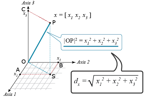
Cluster analyses require a metric that quantifies dissimilarities among all possible pairs of units that we wish to cluster. There are many possible distance metrics that could be used. The most commonly used metric for CA of environments, based on GxE, is the Euclidean distance which is based on the Pythagoras’ theorem (Fig. 8).
Euclidean Distance
For a trait such as yield, it is advisable to first standardize the values so that all of the yield values are on the same scale: Calculate the average and standard deviation for each location, subtract the average value from the genotypic value, and divide by the standard deviation for each of the genotypes by location. Next, calculate the Euclidean Distance of the standardized yield values between all possible pairs of environments.
CA also requires that we choose a grouping algorithm. There are dozens of clustering algorithms, and none should be considered ‘best’ because there are no objective criteria that can be applied to all data sets. For purposes of interpretation using yield data with evidence of GxE, I prefer to use an agglomerative hierarchical clustering technique such as Ward’s (also known as incremental sums of squares) or the Unweighted Pair Group Method with Arithmetic mean (UPGMA, also known as average linkage clustering). Cooper and DeLacy (1994) prefer Ward’s, but for the novice, it is usually good to try several grouping algorithms for purposes of comparison based on the goals of the breeding project.
Variation Flux
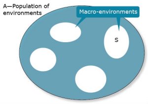
One of the fundamental questions that a breeding project needs to decide is whether to develop broadly adapted cultivars or specific cultivars for specific environments. Often this is determined by production and marketing considerations, but there is also an issue of identifying the types of environments that the crop will encounter within a marketing region. In order to assess the types of environments, the breeder needs to sample the total population of macro-environments using a sample of genotypes. There will clearly need to be trade-offs between these two sampling objectives. Decisions on the trade-offs could actually bias the results that one obtains because genotypic variances can be confounded with GxE variances and vice-versa.
To illustrate, consider Fig. 9, where A represents a population of macro-environments and S is a subset of macro-environments.
Let A serve as our reference population of environments.
It can be shown (with a little algebra) that [latex]\sigma^2_{GA}= \sigma^2_G+\sigma^2_{GS}[/latex]
A consequence is that if the subset population of environments, S, is made more homogeneous (smaller subsets of the total), then genotypic variance will increase because GS interaction variance will decrease. Alternatively, expansion of the targeted subset S of environments will result in a more heterogenous subset which will, in general, increase GS interaction variance at the expense of genetic variance. The challenge is to subdivide an original set of environments so that subdivisions are clearly delineated and substantially more homogeneous. If the market analysis then reveals that multiple sub-environments should be served, it will require an increase in the breeding effort since one breeding program needs to be replaced by multiple breeding projects.
Partition of GxE Variances
GxE variances can be partitioned into two components:
- due to heterogeneity of genotype variance among environments, and
- due to lack of correlation of genetic performance among environments.
Muir et al (1992), provided the means for calculating these two components.
Muir’s Partition Method
Given a model for the phenotype (Equation 5):
[latex]Y_{ijk} = \mu + G_i +E_j+GE_{ij}+\varepsilon_{(ij)k}, \quad i = 1,\ ...\ , g;\ \ j=1,\ ...\ ,e;\ \ k=1,\ ...\ n[/latex]
[latex]\textrm{Equation 5}[/latex] Model for calculating components of phenotype.
where:
[latex]Y_{ijk}[/latex] = phenotype,
[latex]\mu[/latex] = overall mean,
[latex]G_i[/latex] = genotype effect,
[latex]E_j[/latex] = environment effect,
[latex]GE_{ij}[/latex] = genotype by environment interaction effect,
[latex]\varepsilon_{(ij)k}[/latex] = residual (error).
Then SS(GE) is determined as (Equation 6):
[latex]SS(GE)=n\sum^g_i\sum^e_j(\bar Y_{ij.}=\bar Y_{i..}=\bar Y_{.j.}+\bar Y_{...})^2 , \quad =\large \frac{n\sum^g_ {i\neq i'}(S^2_i + S^2_{i'}-2S_{ii'})}{2g};[/latex]
[latex]\text{where, }\quad S^2_i=\sum^e_j(\bar Y_{ij.}-\bar Y_{i..})^2 , \quad S_{ii'}=\sum^e_j(\bar Y_{ij.}-\bar Y_{i..})(\bar Y_{i'j.}-\bar Y_{i'..})[/latex]
[latex]\textrm{Equation 6}[/latex] Model for calculating sum of squares GxE, SS(GE).
where:
[latex]\bar Y_{ij.}[/latex] = mean of ij’s for all plots,
[latex]\bar Y_{i..}[/latex] = mean of i’s for all jk’s,
[latex]\bar Y_{.j.}[/latex] = mean of j’s for all ik’s,
[latex]\bar Y_{...}[/latex] = grand mean,
[latex]S^2_i[/latex] = variance of i,
[latex]S^2_{i'}[/latex] = variance of i’,
[latex]S_{ii'}[/latex] = variance of ii’,
[latex]g[/latex] = all genotypes.
GE Interaction Equation
The GE interaction can then be expressed as:
[latex]\frac{\sum^g_{i i'} \Big[(S_i-S_{i'})^2+2(1-r_{ii'})S_iS_{i'}\Big]}{g}[/latex]
These results then allow the GE interaction sums of squares to be partitioned into a term due to heterogeneous variance, SS(HV)ii’, and that due to imperfect positive correlation of the pair, SS(IC)ii’ (Equation 7).
[latex]SS(HV)_{ii'}=\frac{n(S_i-S_{i'})^2}{g}, \quad SS(IC)_{ii'}=\frac{2n(1-r_{ii'})S_iS_{i'}}{g}[/latex]
[latex]\textrm{Equation 7}[/latex] Model for calculating sum of squares GxE, SS(GE).
where:
[latex]S_i[/latex] = variance of i,
[latex]S_{i'}[/latex] = variance of i’,
[latex]r_{ii'}[/latex] = correlation between i and i’,
[latex]g[/latex] = all genotypes.
Interaction Components
While the first component can be derived from ANOVA results of single environments using the genotypic variance in each environment and their average, the second component can then be calculated using the estimated variance component (EMS) for G x E over all environments and genetic variance component over all environments.
Example Data Sets 1 and 2
To visualize the relative influence of heterogeneity of genotypic responses and lack of correlations among genotypes, consider the following example data sets.
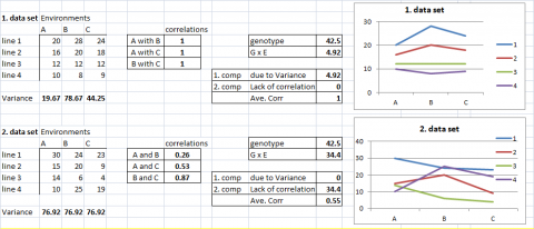
In the first two examples, data sets, G x E is fully explained by one of its two components. In the first case, all G x E is due to the heterogeneity of genotypic variance among environments. In the second case, G x E is completely due to a lack of correlation of genotypic performance among environments.
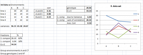
Example Data Set 3
A more realistic example can be found in data set 3, where the GxE is due to a mixture of both components. It is, however, worthwhile to look at their partial contribution; genotypic heterogeneity explains only 18% of GxE interaction, and lack of correlation (consistent ranking) explains 82%.
In the early stages of a breeding project, thousands of genotypes might be evaluated in two or three environments, or a few hundred genotypes might be evaluated in dozens of environments. In such situations, the simple graphical representations (Figs. 2-6) and partitioning of GxE variances (Equations 1-5) become very difficult to interpret.
Alternative Analyses
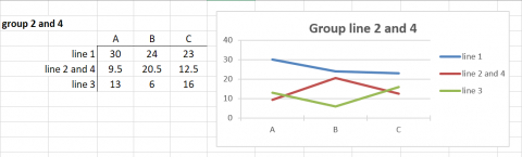
There are alternative analyses and visualization techniques that are used to interpret data from large numbers of genotypes grown in large numbers of environments. For example, pattern analyses employ measures for similarity or dissimilarity to group environments and lines for interpretable graphical representations of either genotypic or environmental performance. Consider the following as illustrated examples based on the data represented in Fig. 11.
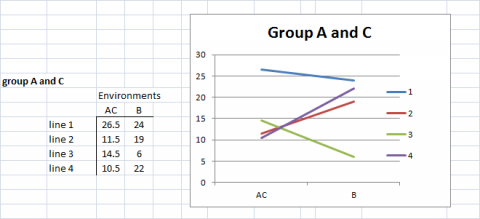
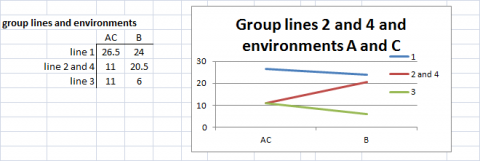
In Fig. 12, we have clustered Environments A and C because the genotypes respond to these environments almost identically and very differently from the manner in which they respond to environment B.
Grouping Similar Responses
In Fig. 12, we also recognize that Genotypes (lines) 2 and 4 respond to the environments in a similar manner, so we cluster these together and represent the response patterns of genotypes as 3 distinct patterns.
Grouping of Lines and Environments
In Figures 12 and 13, either lines or environments are grouped for similar performance. In Fig. 14, both groupings are shown in the same graph. Simple means of groups were taken to give an example for simplification of G x E interactions.
For more complex data sets, measures for similarity and dissimilarity of the performance of genotypes can be used to summarize differences in genetic performance of the genotypes in environments j and j’. We can denote such difference measures as Dg(jj-). We can also consider a measure of a difference, designated as De(ii’-), between environments j and jm, the way in which they discriminate between the genetic performance of genotypes. DeLacy and Cooper (1990) and DeLacy et al. (1990a) discussed alternative forms of De(jj-), which have been used for pattern analysis of relationships among environments in METs (Cooper and Delacey 1994).
Flux between Genotypic Variance and GE Interaction Variance
One of the fundamental questions that a breeding project needs to decide is whether to develop broadly adapted cultivars or specific cultivars for specific environments. Often this is determined by production and marketing considerations, but there is also an issue of identifying the types of environments that the crop will encounter within a marketing region. In order to assess the types of environments, the breeder needs to sample the total population of macro-environments using a broad sample of genotypes. There will clearly need to be trade-offs between these two sampling objectives. Decisions on the trade-offs could actually bias the results that one obtains because genotypic variances can be confounded with GxE variances and vice-versa.
To illustrate, consider Fig. 9 above, where A represents a population of macro-environments and S is a subset of macro-environments.
Let A serve as our reference population of environments.
It can be shown (with a little algebra) that [latex]\sigma^2_{GA} = \sigma^2_G+\sigma^2_{GS}[/latex].
A consequence is that if the subset population of environments, S, is made more homogeneous (a smaller subset of the total), then genotypic variance will increase because GS interaction variance will decrease. Alternatively, expansion of the targeted subset S of environments will result in a more heterogeneous subset which will, in general, increase GS interaction variance at the expense of genetic variance. The challenge is to subdivide an original set of environments so that subdivisions are clearly delineated and substantially more homogeneous. If the market analysis then reveals that multiple sub-environments should be served, it will require an increase in the breeding effort since one breeding program needs to be replaced by multiple breeding projects.
Impact of Multiple Environments
From an introductory course in statistics, we were taught that the phenotypic variance on an entry means basis can be obtained directly from Ordinary Least Squares (OLS) ANOVA by equating the estimated Mean Squares (MS) with Expected Mean Squares (EMS). This is also known as the Method of Moments (MM see Review Module on Statistical Inference). Thus, an estimate of phenotypic variance, [latex]S^2_p[/latex], on an entry mean basis is equal to
[latex]\frac{MS_g}{er}=\sigma^2_g+ \frac{\sigma^2_{ge}}{e}+\frac{\sigma^2_\varepsilon}{er}[/latex]
[latex]\textrm{Equation 8}[/latex] Formula for estimating phenotypic variance on entry mean basis.
where:
[latex]\small MS_{g}[/latex] = mean square value of genotype (g) in the ANOVA table,
[latex]\sigma^2_g[/latex] = genotypic variance,
[latex]\sigma^2_{ge}[/latex] = genotype by environment interaction variance,
[latex]\sigma^2_\varepsilon[/latex] = error variance of the error term, [latex]\varepsilon[/latex],
[latex]r[/latex] = number of replications.
The ability to replicate genotypes and grow them within plots that can be replicated enables the plant breeder to “adjust” their precision around their estimates.
Variance Component Estimation Example
Let us consider a typical plant breeding field trial in which location and year combinations are considered unique environments. (Table 1) Let there be e combinations of years and locations. Also, assume the genotypes, g, are grown at the same locations each year.
| Source | d.f. | Mean Square | EMS |
| Environments (E) | [latex]e-1[/latex] | n/a | n/a |
| Reps within E (R) | [latex]e(r-1)[/latex] | n/a | n/a |
| Genotypes (G) | [latex]g-1[/latex] | M1 | [latex]\sigma^2_e+r\sigma^2_{\bar ge}+re\sigma^2_{\bar g}[/latex] |
| G x E | [latex](g-1)(e-1)[/latex] | M2 |  [latex]\sigma^2_e+r\sigma^2_{\bar g e}[/latex] [latex]\sigma^2_e+r\sigma^2_{\bar g e}[/latex] |
| Residual | [latex]e(g-1)(r-1)[/latex] | M5 | [latex]\sigma^2_e[/latex] |
Estimators
Employing the MM approach, we can obtain estimates of the variance components and, thus, an estimate of the Covariance of the genotypic units (Table 2).
| Function | Variance Estimated |
| [latex]F_2=\frac{(M1-M5)}{r}[/latex] | [latex]\sigma^2_{\bar ge}[/latex] |
| [latex]F_1=\frac{(M1-M2)}{re}[/latex] | [latex]\sigma^2_\bar g[/latex] |
Application Notes
Application of the MM is appropriate only if the data are from a balanced experiment, i.e., the number of genotypic units is the same across reps and environments. In the review chapter, we employed lsmeans to obtain adjusted estimates of entry means in the case of unequal replication per environment. However, we did not learn how to obtain estimates of the variance components for unbalanced data sets.
If there are only a few missing values (say < 5%) from some replicates, then the impact on the estimates of variance components will not be very great. However, we often design experiments to take advantage of seed supplies which may vary greatly among our genotypic units. In such cases, the coefficients of the variance components are not equal to the products of the numbers of reps and environments represented in the EMS. Addressing this issue is fairly straightforward (Milliken and Johnson, 1992). A more difficult problem is that the estimates of the variance components themselves are no longer the “best” estimates. The solution, as described by Holland et al (2003) is to obtain Restricted Maximum Likelihood (REML) estimates in a Mixed Model Procedure (MMP).
References
Cooper, M., and J.H. Delacy. 1994. Relationships among analytical methods used to study genotypic variation and genotype-by-environment interaction in plant breeding multi-environment experiments. Theoretical and Applied Genetics 88: 561–572.
DeLacy, I. H., and M. Cooper. 1990. Pattern analysis for the analysis of regional variety trials. In: Kang MS (ed) Genotype-by-environment interaction and plant breeding. Louisiana State University, Baton Rouge, Louisiana, pp. 301–334.
DeLacy I. H., M. Cooper, and P. Lawrence. 1990a. Pattern analysis over years of regional variety trials: relationship among sites. In: Kang MS (ed) Genotype-by-environment interaction and plant breeding. Louisiana State University, Baton Rouge, Louisiana, pp 189–213.
Holland, J.B., W.E. Nyquist, and C.T. Cervantes-Martínez. 2003. Estimating and interpreting heritability for plant breeding: An update. Plant Breed. Rev. 2003:9–112.
Milliken, G. A., and D. E. Johnson. 1992 Analysis of Messy Data: Vol I, Design Experiments, Chapman & Hall/CRC, London.
How to cite this chapter: Beavis, W., K. Lamkey, K. Espinosa, and A. A. Mahama. 2023. G x E. In W. P. Suza, & K. R. Lamkey (Eds.), Quantitative Genetics for Plant Breeding. Iowa State University Digital Press.
