
Chapter 14: Comparative Mapping and Genomics
Madan Bhattacharyya and Walter Suza
Recall that every cell in a plant contains the same genetic information. The genetic information of a cell constitutes its genome. Therefore, a genome is made up of genes and their regulatory elements. The genome size varies in different species of animals and plants. For example, the human genome is 3.2 Gb while that of hexaploid wheat is 16 Gb. Certainly, a human is very different from a wheat plant. Despite having a smaller genome, a human can think and move but a wheat plant cannot. What then brings about such stark differences? To answer this question we need to compare the genomes of these two organisms for features such as gene content, organization, and function. This type of research is referred to as comparative genomics. Using bioinformatics programs, genome sequences are aligned and the alignments are examined for their evolutionary relationship. Are they homologous, or do they share a common ancestor? Comparative analysis can also be done for genomes of different strains of a species or species that are distantly related. Differences of genomes can therefore be linked to functional consequences, or phenotypes.
- Understand the difference between genetic and physical maps
- Familiarize with comparative genomics tools
- Understand the challenges in comparative genomics
- Familiarize with the application of comparative mapping
Introduction to Structural Genomics
Overview
To conduct comparative genomics we need to know the structure of the genomes we wish to compare. We also need tools/approaches to perform such an analysis. The following sections describe mapping concepts and the fundamentals of comparative genomics.

Genetic Maps
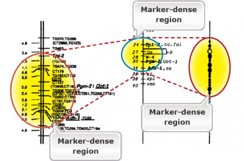
The purpose of genetic maps (also called linkage maps) is to report the length of chromosome intervals, chromosomes, and whole genomes. Genetic maps are based on the rate of recombination. Thus, genetic distances reflect the number of crossover events “observed” for the region, chromosome, or genome of interest. Figure 2 is an example of a genetic map in tomato. Compare the linkage map of molecular markers with the classical genetic map. Molecular markers are super abundance and a single cross allows mapping thousands of markers. Classical maps based on morphological markers are less dense and require integration of maps developed from many crosses. Compare the molecular map with the cytological map on the right. The markers are highly dense in the heterochromatic regions containing the centromeres. This is because of the reduced or suppressed recombination rates in the heterochromatic regions.
Physical Maps
While a genetic map is based on the rates of crossing over and is arbitrary, physical maps provide physical locations of markers. Fluorescence in situ hybridization (FISH) mapping of genetic markers on the pachytene chromosomes can allow us to develop a physical map that corresponds to a genetic map (Fig. 2). Note that in Fig. 2, certain regions are expanded in the genetic map due to higher rates of recombination. The reverse is true for the heterochromatic regions including the centromeres due to reduced recombination rates. Thus, crossover events are not evenly distributed across the chromosomes. Crossover events tend to be suppressed in centromeres and repetitive DNA-rich heterochromatic regions, whereas they are enhanced generally in gene-rich, euchromatic regions. With the sequencing of the entire genomes of crop species, one can now have physical maps of individual chromosomes based on nucleotide sequence. Genome browsers (e.g., Phytozome for soybean) can allow us to navigate the physical maps for gene sequences or molecular markers to the nucleotide level.
Restriction Mapping
Restriction mapping can also allow us to generate a physical map of small DNA fragments cloned in a plasmid vector or larger fragments cloned in BAC (bacterial artificial chromosome) or YAC (yeast artificial chromosome) vectors. This requires determination of the positions of restriction sites on DNA. Consider a piece of linear DNA of 28 kb. The DNA was cut first by HindIII alone, then by PstI alone, and, finally, by both HindIII and PstI together. The following results were obtained:
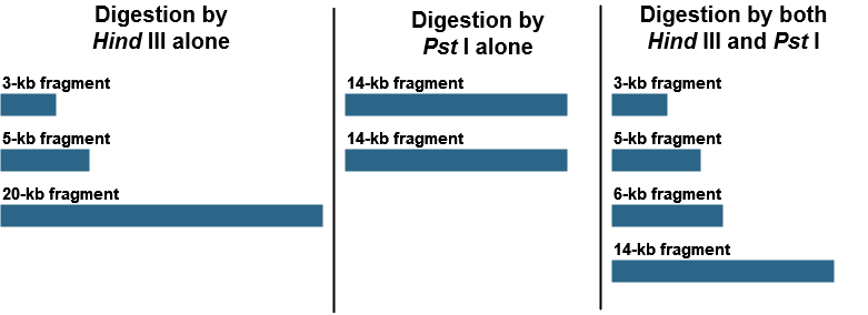
Using these results, draw a map of the HindIII and PstI restriction site on this 28-kb piece of DNA, indicating the relative positions of the restriction sites and the distances between them.
Physical Maps and Genome Sequencing
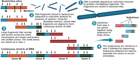
With progress in sequencing technology, an increased number of plant genomes have been sequenced. As a result, physical maps have gained importance. The assembly of the whole-genome sequence relies on both genetic and physical maps for aligning sequenced fragments. Recall in Lesson 5 that BAC and YAC clones are used to prepare genomic libraries for sequencing. The cloned DNA fragments in a YAC or BAC are aligned to form continuous stretches of DNA for subsequent sequencing processes (Fig. 4).
Comparative Mapping
Description
Comparative mapping is a study how the genomes relate across species and genera and even families. The concept started with comparative mapping experiments using RFLP markers between two species that led to the discovery of conserved linear orders of marker loci across related species.
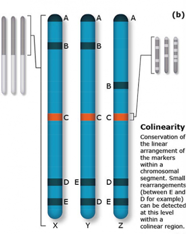
Colinearity and Synteny
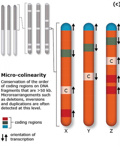
The terms synteny and colinearity have been broadly used to describe the presence of conserved gene orders on chromosomes across species, genera or families. Colinearity describes the conservation of the gene order within a chromosomal segment between different species (Fig. 7). The term colinearity is used to explain conservation of loci at the chromosome level, and micro-colinearity at the locus level (Fig. 8). Synteny was originally used to describe the physical mapping without the linkage assumption. Now the term is used to define chromosomal segments or to gene loci in different organisms located on a chromosomal region originating from a common ancestor (Keller and Feuillet 2000). Genetic loci that arose from a common ancestor are defined as orthologous loci; whereas, paralogous loci are evolved through tandem duplication within a species and located side by side in a chromosomal segment. The examples of colinearity and micro-colinearity are shown in Figures 7 and 8, respectively.
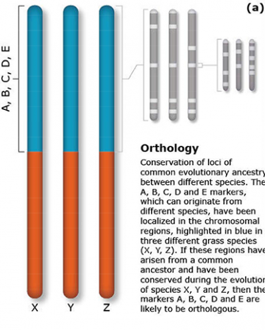
Orthology Example
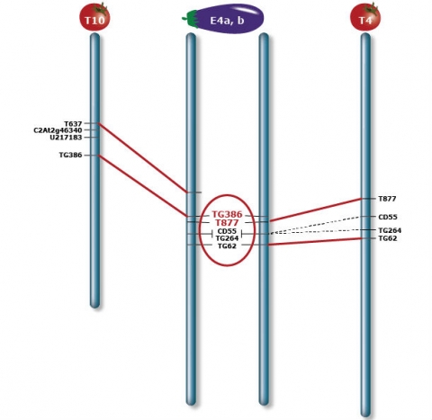
The eggplant chromosome E4 combines two segments (E4a and E4b) orthologous to tomato T4 and T10 respectively, indicating a translocation between the two genomes. The breakpoint is located between markers TG386 and T677 (highlighted in red), and the region is indicated by a black bar beside E4. Orthologous marker pairs are connected by lines. A dash line indicates a marker of low mapping confidence on either or both maps that is not used for deduction of inversions. Vertical arrows beside E4 depict inversions in E4 with respect to T10.
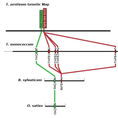
Micro-Colinearity Example
The genetic map of bread wheat (Triticum aestivum) is used to analyze micro-colinearity of the Q locus of T. monococcum, Brachypodium sylvaticum, and rice (Oryza sativa). Genes are shown as colored boxes along the physical maps of each species.
Orthology and Mapping
Comparative mapping is the alignment of chromosomes of related species based on genetic mapping of common DNA markers. Thus, comparative mapping involves the development of linkage maps (Fig. 1). The construction of comparative maps depends on orthology predictions to identify gene pairs of two species. Orthologous loci are loci in different species originating from the same ancestral locus. In contrast, paralagous loci are loci in different (or the same) species that arose due to a duplication of an ancestral locus.
Once the gene pairs have been established, blocks of conserved syteny are established using the positions of each gene in their respective map. The comparative studies in Solanaceae species revealed a modest and consistent rate of chromosomal changes across the family (0.03 ~ 0.12 rearrangements per chromosome per million years). Closely related species showed more conservation of gene orders than the distantly related species. For example, a high conservation of marker orders was observed between tomato and eggplant or tomato and potato than between tomato and pepper. Also, hot spots of chromosomal breakages were identified to suggest that breakpoints are not randomly distributed across the genome. In general, a higher frequency of inversions than translocations was observed among the Solaneaceous species.
Grass Genome Map
Early research to evaluate synteny in grass species suggested the grouping of grasses of the Poaceae families as a single genetic system (Bennetzen and Freeling, 1993). This early synteny work revealed that a large degree of colinearity exists among diverse grasses. For instance, a high conservation across grass species was observed in regions ranging from 5-10 cM. Also, most genes are homologous across species, i.e. all species have essentially the same genes. Additional fine structure mapping revealed insertions of repeated sequences among grass genomes. Overall, these efforts led to the development of the circular grass genome map.
Linear Comparative Map
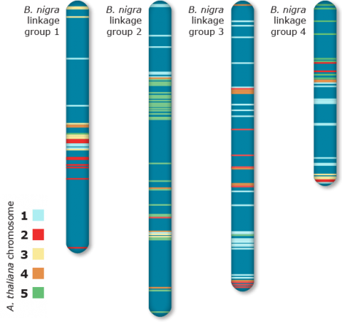
The average conserved segments between Arabidopsis and B. nigra was estimated to be ~8 cMs (Fig. 11). This estimate correspondsto ~90 rearrangements since divergence of the two species; much higher than other species.
Soybean and Arabidopsis Linkage
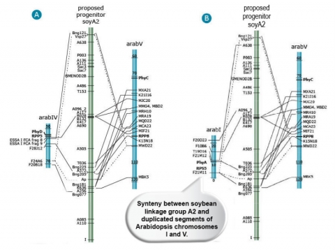
The majority of the comparative mapping studies were based on conservation of nucleotide sequences among closely related species. In 2000, synteny between soybean and Arabidopsis chromosomes was observed when linear orders of predicted protein sequences of genes were compared between the two species (Figure 12). This study also showed that Arabidopsis contains large scale duplicated genomic regions (Grant et al. 2000).
Web-Based Mapping Tools
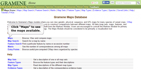
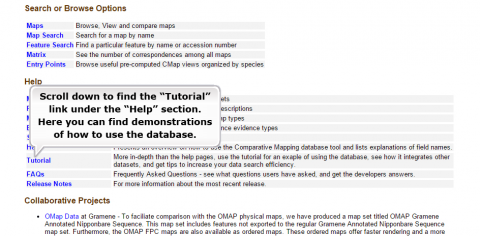
Web-based applications are available for mapping purposes. For example, the Comparative Map Viewer (CMap) available from GRAMENE (Fig. 13) allows comparisons of different maps.
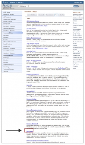
1. In the “Introduction to Bioinformatics” module, you learned about bioinformatics web tools. Go to NCBI and access MapViewer within Genomes & Maps.
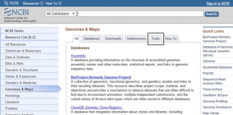
2. In “Introduction to Bioinformatics” module, you learned about bioinformatic webtools. Go to NCBI and access MapViewer within Genomes & Maps.
3. Search for plants, and select Phaseolus vulgaris (kidney bean).
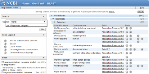
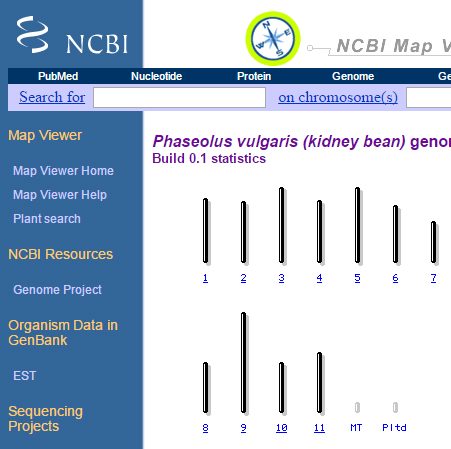
How many chromosomes does kidney bean have?
4. Select chromosome 1, and answer the following:
- How many maps are available for chromosome 1?
- Are the maps physical or genetic? What is the estimated length for each map?
- List the types of markers used to develop each map?
- Try the zoom-in function in the left corner – what do you see?
Comparative Genomics
With the advent of nextgen sequencing, there has been a continuous supply of genome sequence data in the literature. Now the concept of comparing genome maps looking for linear order of genes or synteny has been changed to comparative genomics. It is now feasible to compare related or distant species or genera at the genome level with the aid of available genome sequences. Comparative genomics will have an impact on advancing our knowledge not only in the evolution of crop species, but also in answering biological questions. For example, traditional studies on domestication traits were focused on dozens of loci involved in a variety of functions. Many of the traits were not amenable to study using conventional mapping approaches. Through comparative genomics, it is now known that about 24% of loci in the maize genome were involved in either domestication or subsequent improvement. Through comparative genomics studies, it is now known that in both maize and sunflowers there some loci related to amino acid biosynthesis are enriched. Selection of genes for amino acid biosynthesis during domestication may suggest that protein metabolism has an important role in heterosis. In barley, allelic variation at a flowering time locus in European cultivars appears to have arisen by introgression from barley that was independently domesticated in Central Asia.
Gene Prediction
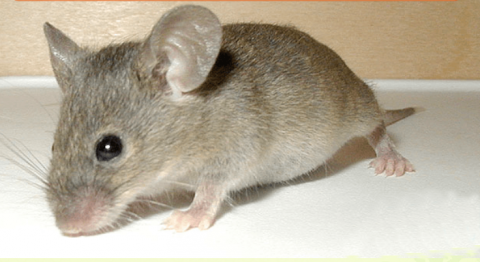
The availability of genome sequence information makes it possible to apply comparative genomics for identification of genes. Gene prediction by comparative analysis involves identification of local similarities by sequence alignment programs in pairs of closely or distantly related genomes. For example, the mouse genome helped increase the accuracy of predicting human genes (Parra et al. 2003).
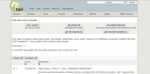
1. Go to the Arabidopsis Information Resource and search for a gene called JAR1.
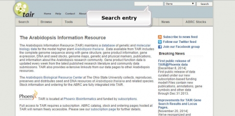
2. What is the function of JAR1 (AT2G46370)?
3. Go to NCBI and search for nucleotide sequence for JAR1 (NM_001202828.1).
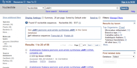
4. Within NCBI, perform a BLAST search for sequences similar to JAR1 (remember to exclude Arabidopsis thaliana in your query). After obtaining sequences producing significant alignments evaluate the four top sequences (maximum identity of 85-99 %). Use your results to answer the following:
- Give the name of the organism from which the sequence was obtained
- Provide the title of the research and the name of the Journal that published the research
- List GenBank id or NCBI reference sequence number of each hit
Detecting Copy Number Variations
The traditional view of comparative genomics was the analysis of synteny (gene order) and sequence comparisons among related species. With the emergence of powerful computational approaches, the examination of the genomic distribution of large insertions and deletions (indels) and copy number variants (CNVs) are becoming the norm.
Copy number variations may result from deletions, causing some individuals to contain only a single copy of a DNA sequence, or may be due to duplications, having certain individuals with more than two copies.
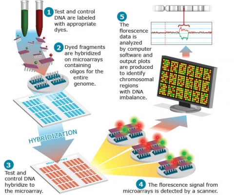
Comparative Genomic Hybridization
Detecting DNA Copy Number Variations
Comparative genomic hybridization (CGH) is a method for genome-wide screening for DNA copy number variations. CGH uses two genomes, a test and a control, which are labeled differentially with fluorescence probes and allowed to competitively hybridize to metaphase chromosomes. The fluorescence signal intensity from test samples compared to controls is plotted across each chromosome, allowing detection of copy number variation. Array-based CGH does not use metaphase chromosomes. Instead, synthetic oligonucleotide probes, or fragments from genomic clones such as BAC or YAC clones are arrayed onto glass slides. The basic method for aCGH is shown in Fig. 18.
Gene Cloning
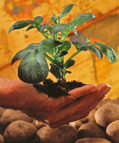
After predicting gene location, the next step is to predict the function of the gene. One of the approaches is to clone the gene using recombinant DNA approaches. Tests for gene function may involve in vitro biochemical analyses for the activity of an enzyme, or complementation of a mutant phenotype by the wild type allele. One can use information from comparative analysis of a species with a simple genome to clone genes from a species with a complex genome. For example, the isolation of the R3a blight resistance gene in potato utilized genomic information from tomato (Huang et al., 2005).
Analysis of Genome Evolution
Evolution of a species is a result of numerous processes including gene duplication and loss, whole genome duplication, variation in ploidy level, retrotransposon activity, and genome rearrangements. Genome evolution describes how the genome has been rearranged through time. Thus, to understand the evolution of a species we need to analyze genome evolution. Genome analysis involves construction of a map in one species and comparison of the map with maps from closely related species by the means of common markers (or common single gene traits).
An understanding of crop origins has long been held as central to the identification of useful genetic resources for crop improvement. The number of times that a species has been domesticated influences the genetic architecture of agronomic traits and the levels of genetic diversity in crop genomes. Domestication shapes the genetic variation that is available to modern breeders as it influences levels of nucleotide diversity and patterns of LD (linkage disequilibrium) genome-wide. The demographic history of domestication also informs our expectations of the genetic architecture of traits and thus our ability to identify causal genetic variants for crop improvement.
Genome Evolution: Details
There is evidence for both single domestications (such as maize and soybeans) and multiple domestications (such as avocados, common beans and barley); but for most crops it is not known whether single or multiple domestication events were involved. Following domestication, extensive admixture with wild relatives may occur; and this may be one explanation for the continued controversy regarding the origins of the domesticated indica and japonica rice.
Isolation of genes encoding domestication traits bears evolutionary importance. Until recently, traits that facilitated domestication, i.e. ‘domestication syndrome’ including decreased dispersal, reduced branching, loss of seed dormancy, reduced natural defenses and increased size of certain morphological features were investigated using mapping strategies. Thus, the study was limited to only a handful traits or loci. Whole-genome data of crops and their wild relatives will facilitate identification of complex demographic histories of many crops. Population genetic approaches, e.g. genome wide association studies (GWAS) will help identify loci that have no known phenotypes; e.g., 2-4% of loci in the maize were affected by artificial selection during domestication. Also, Nextgen sequencing will reveal genome-wide polymorphisms among the accessions leading to discovering demographic history and geographic origins of crop plants.

Domestication and Heterosis
Analysis of Genome Evolution
Comparative genetic mapping studies between species suggested some similarity in the genetic basis of domestication syndrome traits (orthology). Comparative genomics studies in both maize and sunflowers suggest selection on genes for amino acid biosynthesis (unknowingly) during domestication contributes to heterosis.
Challenges: Large Genomes
Most genome tools were not developed for plant genomics studies. First generation molecular markers were isozyme markers that were available in the late 1960s for mapping plant genomes. But such markers are limited in number, and DNA markers paved the way towards construction of high-density molecular maps in 1990s.
Despite the availability of DNA markers, large size of plant genomes remains the greatest challenge in plant comparative genomics.
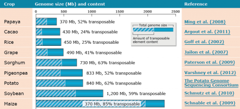
Challenges: Transposable Content
Large genome sizes for plant species are a result of amplification of retrotransposable elements (Fig. 21). In addition, plants genomes contain multi-gene families and paralogous genes that are tandem-duplicated; for example, plant disease resistance genes.
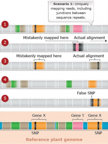
Challenges: Map Assembly: Scenario 1
Duplicated and paralogous sequences, and transposable elements are difficult to assemble during the process of building a genome map (Fig. 22). In Fig. 22 colored shapes represent transposable elements or genes; genes X are a pair of paralogous genes. Short sequence reads are shown directly above where they would map to the reference.
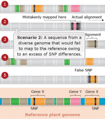
Challenges: Map Assembly: Scenario 2
Duplicated and paralogous sequences, and transposable elements are difficult to assemble during the process of building a genome map (Fig. 23). In Fig. 23 colored shapes represent transposable elements or genes; genes X are a pair of paralogous genes. Short sequence reads are shown directly above where they would map to the reference.
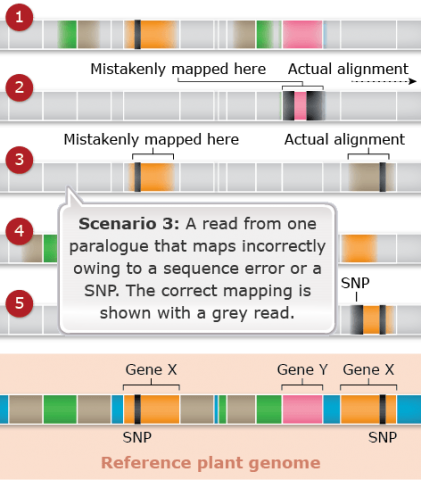
Challenges: Map Assembly: Scenario 3
Duplicated and paralogous sequences, and transposable elements are difficult to assemble during the process of building a genome map (Fig. 24). In Fig. 24 colored shapes represent transposable elements or genes; genes X are a pair of paralogous genes. Short sequence reads are shown directly above where they would map to the reference.
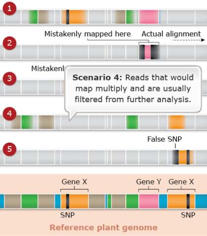
Challenges: Map Assembly: Scenario 4
Duplicated and paralogous sequences, and transposable elements are difficult to assemble during the process of building a genome map (Fig. 25). In Fig. 25 colored shapes represent transposable elements or genes; genes X are a pair of paralogous genes. Short sequence reads are shown directly above where they would map to the reference.
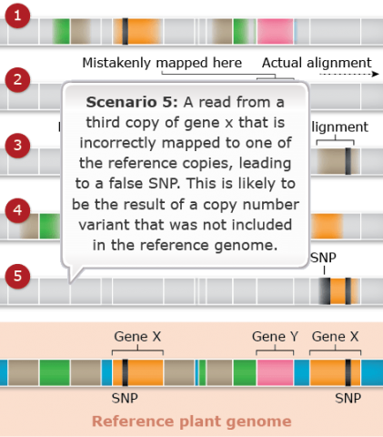
Challenges: Map Assembly: Scenario 5
Duplicated and paralogous sequences, and transposable elements are difficult to assemble during the process of building a genome map (Fig. 26). In Fig. 26 colored shapes represent transposable elements or genes; genes X are a pair of paralogous genes. Short sequence reads are shown directly above where they would map to the reference.
Challenges: Repeated
Sequences
High proportion of repeated sequences also makes it difficult to conduct reference genome-based SNP identification and genome-wide association studies. Therefore, regardless of the emerging high throughput sequencing technologies, it remains challenging to achieve sufficient genome coverage for assembling short read sequences and paralogous sequences. Consequently, fewer crop species with large genomes have been sequenced so far. Improvement in sequence read length by nextgen approaches will reduce this problem allowing detection of local patterns of LD for identifying paralogous reads in complex crop genomes.
Summary
Comparative genomics is a field of research focusing on determining the evolutionary relationships of genomes and link differences to functional consequences, or phenotypes. With progress in sequencing technology, an increased number of plant genomes have been sequenced making it possible to construct comparative maps and predict gene pairs of two species. To understand how genomes evolve, a genome map is constructed in one species and compared with maps from closely related species by the means of common markers. The majority of the comparative mapping studies are based on conservation of nucleotide sequences among closely related species. Comparative genomics is also useful for the identification of genes. Following prediction of gene location by comparative analysis, target genes may be isolated and characterized to determine their function. However, one of the greatest challenges in plant comparative genomics is the large size of plant genomes. Consequently, fewer crop species with large genomes have currently been sequenced.
References
Argout et al. 2011. The genome of Theobroma cacao. Nat. Genet. 42:101-109.
Bennetzen, J. L., and M. Freeling. 1993. Grasses as a single genetic system: genome composi-tion, collinearity and compatibility. Trends Genet. 9: 259-261.
Dubcovsky, J. 2001. Plant gene cloning may lead to better timing of flowering. NRI research highlights 2001 No. 2.
Fan, C., M. D. Vibranovski, Y. Chen, and M. Long. 2007. A Microarray Based Genomic Hybridiza-tion Method for Identification of New Genes in Plants: Case Analyses of Arabidopsis and Oryza. J. Integr. Plant Biol. 49:915-926.
Faris, J. D., Z. Zhang, J. P. Fellers, and B. S. Gill. 2008. Micro-colinearity between rice, Brachypodi-um, and Triticum monococcum at the wheat domestication locus Q. Funct. Integr. Genomics 8:149-164.
Feuillet, C., and B. Keller. 2002. Comparative genomics in the grass family: Molecular charac-terization of grass genome structure and evolution. Ann. Bot. 89: 3-10.
Gale, M. D., and K. M. Devos. 1998. Comparative genetics in the grasses. Proc. Natl. Acad. Sci. USA 95:1971-1974.
Goff et al. 2002. A draft sequence of the rice genome (Oryza sativa L. ssp. Japonica) Science 296:92-100.
Grant, D., P. Cregan, and R. C. Shoemaker. 2000. Genome organization in dicots: Genome duplica-tion in Arabidopsis and synteny between soybean and Arabidopsis. Proc. Natl. Acad. Sci. USA 97:4168–4173.
Huang, S., E. A. G. van der Vossen, H. Kuang, et al. 2005. Comparative genomics enabled the isolation of the R3a late blight resistance gene in potato. Plant J. 42:251-261.
Iovene, M., S. M. Wielgus, P. W. Simon, et al. 2008. Chromatin structure and physical mapping of chromosome 6 of potato and comparative analyses with tomato. Genetics 180:1307-1317. Epub 2008 Sep 14.
Jaillon et al. 2007. The grapevine genome sequence suggests ancestral hexaploidization in ma-jor angiosperm phyla. Nature 449:463-468.
Keller, B., and C. Feuillet. 2000. Colinearity and gene density in grass genomes. Trends Plant Sci. 5:246–251.
Lagercrantz, U. 1998. Comparative Mapping Between Arabidopsis thaliana and Brassica nigra Indicates That Brassica Genomes Have Evolved Through Extensive Genome Replication Accom-panied by Chromosome Fusions and Frequent Rearrangements. Genetics 150:1217-1228.
Ming et al. 2008. The draft genome of the transgenic tropical fruit tree papaya (Carica papaya Linnaeus) Nature 452:991-997.
Morrell P. L., E. S. Buckler, and J. Ross-Ibarra. 2012. Crop genomics: advances and applications. Nature Reviews 13:85-96.
Parra, G., P. Agarwal, J. F. Abril, et al. 2003. Comparative gene prediction in human and mouse. Genome Res. 13:108-117.
Paterson et al. 2009. The Sorghum bicolor genome and the diversification of grasses. Nature 457:551-556.
Pierce, B.A. 2010. Genetics: A conceptual approach. Macmillan: 559-580.
Sarkar, S. F., J. S. Gordon, G. B. Martin, and D. S. Guttman. 2006. Comparative Genomics of Host-Specific Virulence in Pseudomonas syringae. Genetics 174:1041-1056.
Scmutz et al. 2010. Genome sequence of the palaeopolyploid soybean. Nature 463:178-183.
Schnable et al. 2009. The B73 genome: Complexity, Diversity, and Dynamics. Science 326:1112-1115.
Tanksley, S. D., M. W. Ganal, J. P. Prince JP, et al. 1992. High density molecular linkage maps of the tomato and potato genomes. Genetics. 132:1141-1160.
The Potato Genome Sequencing Consortium. 2011. Genome sequence and analysis of the tuber crop potato. Nature 475:189-197.
Varshney et al. 2012. Draft genome sequence of the pigeonpea (Cajanus cajan) an orphan leg-ume crop of resource-poor farmers. Nature Biotechnol 30:83-92.
Wu, F., and S. D. Tanksley. 2010. Chromosomal evolution in the plant family Solanaceae. BMC Genomics 11: 182-193.
Zhu, H., H. Choi., D. R. Cook., and R. C. Shoemaker. 2005. Bridging model and crop legumes through comparative genomics. Plant Physiol 137: 1189-1196.
