
Chapter 3: Modeling and Data Simulation
Thomas Lübberstedt; William Beavis; and Walter Suza
The main objective of plant breeding is to develop new cultivars that are genetically superior to those presently available across a range of environmental conditions. However, to a large extent, conventional breeding relies heavily on phenotypic selection and the skill of the breeder. Increasing production of genomic data and better methods to phenotype plants provide an opportunity to evaluate important traits in plants. Computer simulation can help to utilize the large and diverse pool of genetic data to build appropriate models to predict the performance of testcrosses based on pre-existing information, and to compare different and establish optimal selection methods in plant breeding. In this module, computer simulation tools available to plant breeders and geneticists will be introduced. This module will include examples of computer simulation for crop genetic improvement. In the last part of this module, you will learn how to conduct a simple simulation study.
- Familiarize with genetic simulation tools
- Familiarize with simulation modeling
- Learn to design simulation experiments for plant breeding
Genetic Simulation Tools
Methods and Processes
Natural or artificial methods and processes are modeled for purposes of predicting unknown outcomes. In plant breeding, simulation models are used to choose among proposed breeding methods because experimental evaluation of breeding methods is time and resource limited.
Modern computers are designed to possess greater computational power and data storage space at a reduced price. With the recent explosion in production of genomic data, custom designed programs will provide opportunity for data analysis and simulation to improve plant breeding methods. Examples of publicly available simulation software for plant breeding, software functionality, and assumptions made in modeling are summarized in the next pages.
A. Plabsoft
Plabsoft is a computer program used to analyze data and build simulations based on various mating systems and selection strategies. Plabsoft uses the following model:
[latex]G =\sum\limits_{S \subseteq N} X_{S}[/latex]
where:
G = genotypic value
Xs = genetic haplotype effect at a subset of loci S
N = loci set
An article describing how population simulation and data analysis can be conducted using Plabsoft was published in 2007 by Maurer, Melchinger, & Frisch.
B. QU-GENE
QU-GENE is a computer program used to estimate epistatic and G x E effects using the E(N:K) genetic model.
where:
E = the number of types of environments
N = the number of genes
K = level of epistasis.
Parentheses in the model indicate that different N:K genetic models can be “nested” within types of environments. More information on the QU-GENE platform is found in this article by Podlich & Cooper (1998).
Information on the use of computer clusters for large QU-GENE simulations was later published by
C. MBP
MBP is a computer program used in optimizing resource allocation to maximize genetic gain in breeding of hybrid maize using doubled haploid techniques. MBP uses the following model:
[latex]\sigma _{t}^{2}=\sigma _{GCA}^{2}+\sigma _{SCA}^{2}/T[/latex]
where:
σ2 = estimated genetic variance between test cross progenies
σ2GCA and σ2SCA = derivatives of additive and dominance variance estimates
T = the number of testers
Read more about the MBP software in Gordillo & Geiger (2008).
D. GREGOR
GREGOR is a computer program used to predict the mean result of mating and selection in plant breeding. GREGOR is implemented in the MS-DOS environment and does not require use of empirical data. All inputs including individual, trait, and marker data are simulated by the program. GREGOR can create files that are compatible for Mapmaker/Mapmaker QTL programs.
E. PLABSIM
PLABSIM is a computer program used for simulation of marker-assisted backcross methods.
F. GENEFLOW
GENEFLOW provides a platform for determining the nature and structure of genetic diversity by integrating pedigree, genotype, and phenotype data. Simple statistical analyses, such as ANOVA, regression, t tests and correlations are supported in GENEFLOW. Go to this link to access GENEFLOW
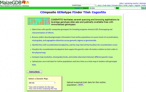
G. COGENFITO
The composite genotype finder tool (COGENFITO) is a web-based program used as a search tool for identification of specific genotypes (Fig. 2).
H. AlphaSim
AlphaSim is a software used to perform simulations for breeding programs. AlphaSimR uses scripting to build simulations for commercial breeding programs.
Summary of Programs and Functionality
Functionality and Assumptions of Computer Software Programs
Software: Plabsoft
- Assumptions: Absence of selection in the base population; random mating; infinite population size; no crossover interference
- Models: Quantitative genetic model; count location model
- Functionality: Integrates population genetic analyses and quantitative genetic models for estimating genetic diversity; tests HWE and calculates LD; haplotype-block-finding algorithms to predict hybrid performance
Software: QU-GENE/QuLine
- Assumptions: No mutation; no crossover interference; all random terms normally distributed
- Models: E(NK) model; Infinitesimal model
- Functionality: Employs simple to complex genetic models to mimic inbred breeding programs, including conventional selection and MAS
Software: MBP
- Assumptions: Timely staggered breeding cycles; no epistatic and maternal effects; no correlated response in test cross performance; infinite population size to calculate selection intensity
- Models: Quantitative genetic model for optimization; Infinitesimal model
- Functionality: Optimizes hybrid maize breeding schemes based on DH lines and maximizes the expected genetic gain per year by means of quantitative genetic model calculations under the restriction of a given annual budget
Software: GREGOR
- Assumptions: No crossover interference; no epistatic effect
- Models: Quantitative genetic model
- Functionality: Predicts the average outcome of mating or selection under specific assumptions about gene action, linkage, or allele frequency
Software: PLABISM
- Assumptions: No crossover interference
- Models: Random-walk algorithm to simulate crossovers during meiosis
- Functionality: Simulates marker-assisted introgression of one or two target genes using backcrossing
Software: GENEFLOW
- Assumptions: Diploid inheritance
- Models: Genotype; Pedigree; Population and Report modules; optional Multiplex and Germplasm
- Functionality: Studies nature and structure of genetic diversity
Software: COGENFITO
- Assumptions: Maize only/li>
- Models: Security modules, Genome model limited to marker maps in MaizeGDB
- Functionality: Screens marker data from a given genetic mapping population to identify line with user-defined informative haplotypes
Applying Computer Simulation
Computer Simulations
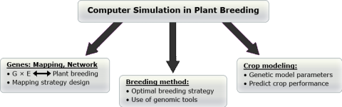
Computer simulations were used as early as 1957 to solve theoretical problems in population genetics that are intractable using conventional algebraic and statistical approaches (Fraser and Burnell, 1970). Substantial time and field resources are needed to conduct field experiments to compare breeding efficiency from different selection strategies to predict cross performance using available gene information. The power of computer simulation is the ability to sample as many conditions as possible beyond the breeder’s capability of solving them by hand. Taking advantage of the speed and efficiency of sampling by computers, breeders have found a tool that can be used to test models and provide more confidence in the performance of the model in the field environment. The major applications of computer simulation in crop genetic improvement are indicated in Fig. 3.
Examples of Application of Computer Simulation in Plant Breeding
Example 1: Evaluating plant breeding strategies
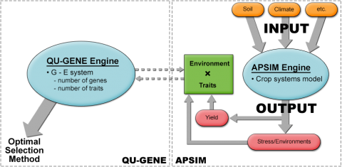
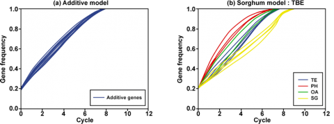
Chapman et al. (2003) simulated the S1 recurrent selection method for sorghum in three drought environment types in Australia. The assumption was that 15 genes influence yield in sorghum by controlling several traits including, transpiration efficiency coefficient, flowering time, osmotic adjustment, and stay green traits (Chapman et al. 2003). In this work, QU-GENE was linked with Agricultural Production Systems sIMulator (APSIM) program (Fig. 4) to simulate the breeding population and the corresponding trait values for each genotype. As mentioned earlier, QU-GENE helps determine gene effects, G x E interactions, and epistasis (Podlich and Cooper, 1998). Therefore, combining QU-GENE with APSIM helps determine the importance of the interactions detected by QU-GENE on yield in target environments.
Findings
The data in Fig. 5 suggest that for different combinations of traits being tested in particular environments, the fixation of certain traits may not occur until one or more other traits have been improved. While in Fig. 5a the rate of gene fixation is similar, in Fig. 5b, the genes are fixed at different rates. To the breeder, it is important to fix all desirable alleles at the same rate so that desirable level of homozygosity is attained in earlier generations.
Example 2: Efficiency of Marker-Assisted Selection
Hospital et al. (1997) investigated the relative efficiency (RE) of marker-assisted selection (MAS) based on an index consisting phenotypic value and molecular score of individuals (Cluster Analysis, Association & QTL Mapping). In this example, the phenotypic value of (Pi) of individual i was computed as the sum of its genotypic (Gi) and environmental (Ei) values:
[latex]P_{i}=G_{i}+E_{i}[/latex]
One of the assumptions is that the environmental value is a random normal variable with mean 0 and variance σ2E. The genetic value was computed as:
[latex]G_i = \sum_{q = 1}^{nq}x_q\Theta _{iq'}[/latex]
where:
Xq = effect of QTL q
Ɵiq = the number of favorable alleles carried by individual i at locus q
nq = total number of QTL (for this study 25 QTLs were considered)
Finding 1
- The genetic variances at the QTL in the original F2 follow a geometric series
- There is no genetic interference in recombination
Findings
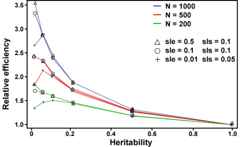
- The relative efficiency of MAS depends on population size (Fig. 6). At low heritabilities, the larger the population size, the higher the RE of MAS.
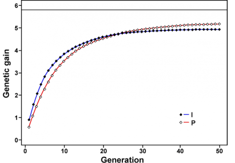
Finding 2
- MAS is less efficient than phenotypic selection in the long term (Fig. 7).
How to Design a Simulation Experiment
New Breeding Methods
The future success of plant breeders will depend upon their abilities to propose and evaluate new breeding methods. The motivation to succeed will rely on the breeder’s ability to predict cross performance by developing and validating new statistical methods, and evaluating new breeding processes. This will require application of models to simulate the methods or processes, and to evaluate the methods based on appropriate criteria, for example, accuracy, power, precision, efficacy, and efficiency (e.g., genetic gain).
Models are used to represent, describe and quantify natural phenomena, and can be arbitrarily simple depending upon their purpose. For example, consider two cultivars (1 and 2) of a crop species. Our task is to (a) describe how the two cultivars might be the same and/or different, and (b) how to test whether the two cultivars are the same. The following statistical model can be used to compare quantitative differences (e.g., yield) of the two cultivars (Table 1).
[latex]Y_{ij} = \mu + C_i + \varepsilon_{(i)j}[/latex]
where:
Yij = observation for the ith cultivar entry at the jth location
[latex]\mu[/latex] = an overall mean
Ci =an effect due to the ith cultivar entry
[latex]\varepsilon_{(i)j}[/latex] = a random error associated with the response of ith cultivar entry at the jth location
i = 1
j = 1
| Cultivar | 1 | 2 | 3 | 4 | 5 | Total | Mean |
|---|---|---|---|---|---|---|---|
| 1 | 19 | 14 | 15 | 17 | 20 | 85 | 17 |
| 2 | 23 | 19 | 19 | 21 | 18 | 100 | 20 |
Assumptions of the Model
- Effects are additive
- Errors are normally distributed, homogeneous, and independent
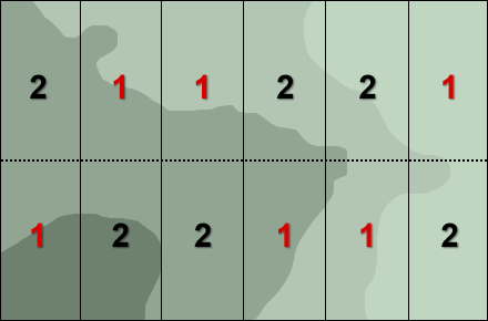
In a field experiment it would be possible, as a result of randomization for all the plots with one of the cultivars to be grouped together in one corner of the experimental plot (Fig. 8). With spatial variability in soil fertility and moisture content possible this might lead to misleading results.
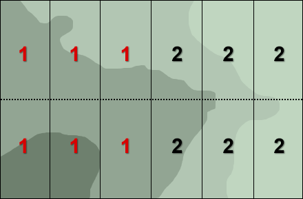
One of the remedies to address such spatial field variability (Fig. 8) is to group the units (blocks) such that units in the same group are as similar as possible, and then allocate at random each cultivar to one unit each of the groups (Fig. 9).
New Field Experiment Design
The new design (Fig. 9) allows the application of the following model:
[latex]Y_{ijk} = \mu + B_j + C_i + \varepsilon_{(ij)k}[/latex]
where:
Yijk = observation for the kth replicate of the jth block of the ith cultivar
μ = an overall mean
Ci = an effect due to the ith cultivar entry
ε(ij)k = a random error associated with the response of the kth replicate of the ith cultivar in the jth block
Bj = an effect due to the jth block
k = 1
Simulate a Double Haploid Population
An Example for Simulating a Double Haploid (DH) Population in Excel
Goal: create phenotypic values for 30 DH genotypes in Excel; a model for the phenotypic performance of these lines includes the population mean, a single gene with an additive effect of +1 or -1 (G), equal environmental effect (E = +1) for all 30 DH genotypes, no genotype x environment interactions (GxE), and a normally distributed error.
Thus the model is Phenotype = Mean + Genotype + Environment + GxE + Error.
Excel Exercise:
To create a simulated population of 30 DH genotypes in Excel, these are the steps:
- In column A (Lines), provide line numbers 1-30. Type a “1” in field A4 and a “2” in A5. Mark both fields with the mouse, and drag down the bottom right corner of the box around fields A4 and A5 to field A33. This will create numbers 1-30 in sequence within this column in fields A4-A33.
- In column B (Environment, Env): type a “1” in field B4. Mark this field and drag down to B33. All fields will in this case show a value of 1.
- In column C (Mean): type a “150” (bushels per acre). Proceed like in column B, so that all 30 DH genotypes get the same mean value of 150.
- In column D (Genotype, G), add the following command in field D4: “= IF(RAND()<0.5,-1,1)”. “RAND()” will generate random numbers in the interval of 0 to 1. Thus, the expression “IF(RAND()<0.5, -1,1)” will generate a value of -1, when a random number below 0.5 is generated (in 50% of the cases). This expression will generate a value of +1 in the other 50% of the cases. By entering this command in field D4, and then dragging down to D33, random numbers -1 or 1 will be added in the fields D4 to D33.
- In column E (GxE): type a “0” in field E4. Mark this field and drag down to E33. All fields will in this case show a value of 0.
- In column F (Error), add the following command in field F4: “= NORM.INV(RAND(),0,1)”. his command will create normally distributed random numbers. The Excel NORMINV function calculates the inverse of the Cumulative Normal Distribution Function for a supplied value of x, and a supplied distribution mean (0 in this case) & standard deviation (1 in this case). This information and further useful information on functions in Excel can be found under the Excel “Help function”. When opening this Help function by clicking on the “?” symbol, information on functions can be accessed in various ways, e.g., by searching an alphabetical list of functions.
- The Phenotype can be determined in column I, by adding the following command in field I4: “=SUM(C4:F4)”. This will add for DH genotype 1 the values in fields C4 to F4, which according to the model adds up to the Phenotype of this genotype. By dragging down to I33, this summation will be conducted for all 30 DH genotypes.
- Additional, new simulations of Phenotypes for 30 DH genotypes are obtained by marking fields I4-I33, and copying those into a new column (e.g., K4-K33). By repeating this copy and paste step, multiple sets of 30 DH genotypes can be simulated in a short time.
Possible Uses
Assume, a genetic marker for the gene with additive effect of -1 or +1 is available and co-segregating with that gene. It could be evaluated, how often a t-test would indicate a significant difference between the two genotype classes, in other words, it would enable to determine the power of detecting a gene with this effect, in a DH population of this size. Generally, respective simulation studies can be used to determine the power of detecting a known effect, and thus help to design proper experiments in terms of population size, number of environments, etc. The limitation is, that simulation studies have to make assumptions about unknown effects.
References
Chapman, S., M. Cooper, D. Podlich, and G. Hammer. 2001. Evaluating plant breeding strategies by simulating gene action and dryland environment effects. Agron J. 95: 99-113.
Frisch, M., M. Nohn, and A. E. Melchinger. 2009. PLABSIM: Software for simulation of marker-assisted backcrossing. J. Heredity 91: 86-87.
Gordillo, G. A., and H. H. Geiger. 2008. MBP (Version 1.0): A software package to optimize maize breeding procedures based on doubled haploid lines. J Heredity 99: 227-231.
Hospital, F., L. Moreau, F. Lacoudre, A. Charcosset, and A. Gallais. 1997. More on efficiency of marker-assisted selection. Theor. App. Genet. 95: 1181-1189.
Jiankang Wang. 2012. Modelling and Simulation of Plant Breeding Strategies, Plant Breeding, Dr. Ibrokhim Abdurakhmonov (Ed.), ISBN: 978-953-307-932-5, InTech, DOI: 10.5772/27863.
Li, X., C. Zhu., J. Wang, and J. Yu. 2012. Computer simulation in plant breeding. Advances in Agronomy 116: 219-264.
Maurer, H. P., A. E. Melchinger, and M. Frisch. 2008. Population genetic simulation and data analysis with Plabsoft. Euphytica 161: 133-139.
Micallef, K. P. M. Cooper, and D. W. Podlich. 2001. Using clusters of computers for large QU-GENE simulation experiments. Bioinformatics 17: 194-195.
Podlich, D. W., and M. Cooper. 1998. QU-GENE: a simulation platform for quantitative analysis of genetic models. Bioinformatics 14: 632-653.
Sun, X., T. Peng., and R. H. Mumm. 2011. The role and basics of computer simulation in support of critical decisions in plant breeding. Mol Breeding 28: 421-436.
Tinker, N. A., and D. E. Mather. 1993. GREGOR: Software for genetic simulation. J. Heredity 84: 237.
