
Chapter 2: Markers and Sequencing
Thomas Lübberstedt; Madan Bhattacharyya; and Walter Suza
Mutations are the ultimate source of all genetic variation. Mutations can occur at all levels of genetic organization, classified as gene, chromosome or genome mutations. Gene and chromosome mutations are discussed in this lesson. Gene mutations involve nucleotides or short DNA segments (one or few nucleotides substituted, inserted, or deleted). Chromosome mutations are large-scale chromosome alterations including deletions, insertions, inversions, and translocations. Genome mutations – involving changes in number of whole chromosomes or sets of chromosomes.
Genetic variation – dissimilarity between individuals attributable to differences in genotype – that is generated by mutations is acted upon by various evolutionary forces. Evolutionary processes that alter species and populations include selection, gene flow (migration), and genetic drift – whether plants are cultivated or wild. Evolution can be defined as a change in gene frequency over time. The way that plants evolve is dependent on both genetic characteristics and the environment that they face.
- Understand the importance of DNA sequence variation within species
- Learn the principles of sequencing
- Understand next generation (nextgen) sequencing
- Understand nextgen sequencing bioinformatics
- Understand prerequisites, prospects, and limitations in using sequencing for genotyping
- Understand the concept of imputation
- Understand RFLP, SSR, and AFLP as examples of classical markers
- Understand SNP and INDEL marker basics
- Understand two basic applications of markers: fingerprinting and gene-tagging
- Understand underlying technologies of non-DNA marker systems and strengths and weaknesses of non-DNA versus DNA markers
Genetic Variation
Genetic variation results from differences in DNA sequences and, within a population, occurs when there is more than one allele present at a given locus. Changes in gene frequencies within populations caused by natural selection can lead to enhanced adaptation, while changes caused by human-directed selection can facilitate development of useful genetic variability and selection of superior genotypes. Selection is the differential reproduction of the products of recombination — both within and between chromosomes.
The basic tools used to characterize genetic variation within and between populations are called genetic markers. Markers can be visible traits, proteins, genes, DNA sequences, or RNA sequences, and can be genetically mapped to a particular chromosomal location. They can be used to track the inheritance of nearby genes to which they are closely linked. A marker may be part of a gene itself or more commonly in a chromosome segment close by a gene of interest. Markers are characteristically locus-specific and polymorphic (i.e., segregating) in the population under study, and also have easily observable phenotypes. Markers allow determination of alleles present in individuals or populations.
Principles of Sequencing
Historically, plant breeders seeking sources of variability were constrained in choice of parental materials or plant genetic resources that were interfertile through the process of recombining locally adapted plant materials via sexual reproduction within closely related gene pools or just by evaluation and selection of particular desirable, existing genotypes to produce improved plant varieties. But a range of new techniques such as mutation induction, genetic engineering (transgenic or transformed plants), and in vitro methods (somatic cell hybridization, tissue culture, doubled haploids, induced polyploids) expand the source and scope of variability that can be used in crop improvement.
Our expanding understanding of the molecular basis of genetics has provided insights and technologies that further not only our basic understanding of genes and their regulation, but also provide additional tools for crop improvement. Molecular techniques enable breeders to generate genetic variability, transfer genes between unrelated species, move synthetic genes into crops, and make selections at the molecular, cellular, or tissue levels. Combining these laboratory techniques with conventional field approaches can shorten the time and reduce the costs for developing improved cultivars. The importance and application of molecular technologies are rapidly increasing.
Sequencing Efforts
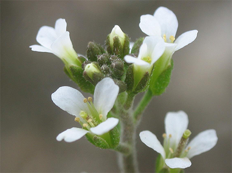
Sequencing is the determination of the order of the nucleotides on a DNA molecule. A major milestone in plant biology was reached when the genome of Arabidopsis thaliana was published (The Arabidopsis Genome Initiative, 2000). Thereafter, the scientific community pursued the genomes of several crop plants used for feed and food. This effort attempts to keep a current list of sequenced plant genomes.
| Common name | Scientific name | Year |
|---|---|---|
| Potato | Solanum tuberosum | 2011 |
| Grape | Vitis vinifera | 2007 |
| Cucumber | Cucumis sativus | 2009 |
| Popular | Populus trichocarpa | 2006 |
| Strawberry | Fragaria vesca | 2010 |
| Castor bean | Ricinus communis | 2010 |
| Apple | Malus x domestica | 2010 |
| Cannabis | Cannabis sativa | 2011 |
| Lotus | Lotus japonicus | 2008 |
| Soybean | Glycine max | 2010 |
| Pigeon pea | Cajanus cajan | 2011 |
| Chocolate | Theobroma cacao | 2010 |
| Papaya | Carica papaya | 2008 |
| Arabidopsis | Arabidopsis thaliana | 2000 |
| Arabidopsis | Arabidopsis lyrata | 2011 |
| Various | Brassica rapa | 2011 |
| Thellungiella | Thellungiella parvula | 2011 |
| Date palm | Phoenix dactylifera | 2011 |
| Rice | Oryza sativa L. | 2002 |
| Brachy | Brachypodium distachyon | 2010 |
| Maize | Zea mays | 2009 |
| Sorghum | Sorghum bicolor | 2009 |
| Moss | Physcomitrella patens | 2008 |
| Selaginella | Selaginella moellendorffii | 2011 |
Sanger’s Dideoxy DNA-Sequencing Procedure
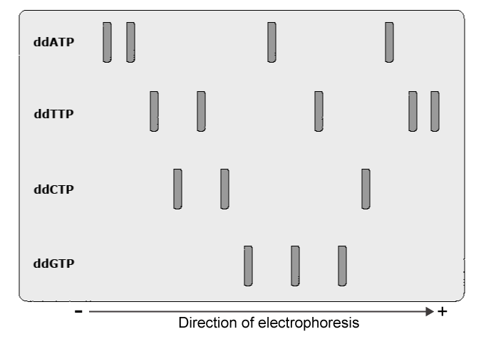
This procedure was developed by Fred Sanger in the 1970s. Sanger, along with Walter Gilbert, won the Nobel Prize in chemistry in 1980 for their sequencing developments. The method uses enzymatic reactions to incorporate specific terminators of DNA chain elongation called 2′,3′-dideoxynucleoside triphosphates (ddNTPs). The ddNTP molecules can be incorporated into the growing DNA chain through their 5′ triphosphate groups. However, because they lack a hydroxyl (OH) groups on the 3′-C of the sugar moiety, they cannot form a phosphodiester bond with deoxynucleotide triphosphates (dNTPs) during the sequencing reaction, resulting in termination of DNA chain elongation.
Sequenced Plant Species
Additional Resources
- An updated overview of sequenced plant genomes is available from the NIH National Library pf Medicine’s Genome data package.
- Johnny Clore has developed a useful YouTube video describing Sanger DNA sequencing.
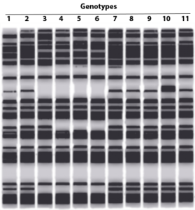
The figure below shows gel electrophoresis sequencing results based on the dideoxy method. Examine the banding pattern and describe the order of the nucleotides of the original template strand.
Maxam & Gilbert Procedure
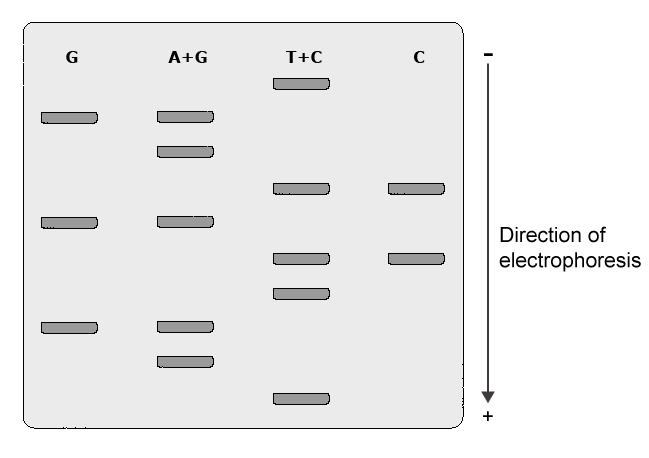
This procedure was developed by Allan Maxam and Walter Gilbert in 1977. The Maxam & Gilbert procedure is based on chemical degradation of DNA chains. In this procedure, a segment of DNA is labeled at one end with a radioactive label (32P ATP). A solution containing the labeled DNA is distributed into four different tubes. A chemical that specifically destroys one or two of the four bases (G, A+G, C, C+T) in the DNA is added into each tube. Addition of the chemical piperidine to the DNA results in cleavage of the strand at the position of the modified base. The length of the cleaved fragments depends on the distance between the modified base and the labeled end of the DNA segment. The cleaved products of each of the four reactions (G, A+G, C, and C+T) will be evaluated by autoradiography and the banding pattern on film is scored to determine the DNA sequence.
Next Generation Sequencing
Definition
Next generation sequencing is defined as a high-throughput sequencing method that combines parallel processes to produce millions of sequences at once. Several nextgen technologies are currently in use. The lesson focuses on the following technologies: pyrosequencing, Illumina, SOLiD, single molecule real time, and ion torrent sequencing.
Pyrosequencing or 454 Sequencing
454 sequencing was developed by Roche and uses a procedure known as sequencing by synthesis, or pyrosequencing.
SOLiD
The SOLiD system was developed by Life Technologies and is based on a technique of oligonucleotide ligation and detection. Like pyrosequencing, SOLiD sequencing begins with fragmented DNA on an agarose bead.
Illumina
The Illumina system uses a terminator-based method to detect single bases as they are incorporated into a growing DNA strand.
SMRT Sequencing
Single-Molecule Real-Time (SMRT) system was developed by Pacific Biosciences and uses a polymerase based approach to sequence single DNA molecules in real-time. The technique works similarly to 454 pyrosequencing, but it uses a luminous dye attached to the phosphate chain of each nucleotide.
Third-Generation Sequencing
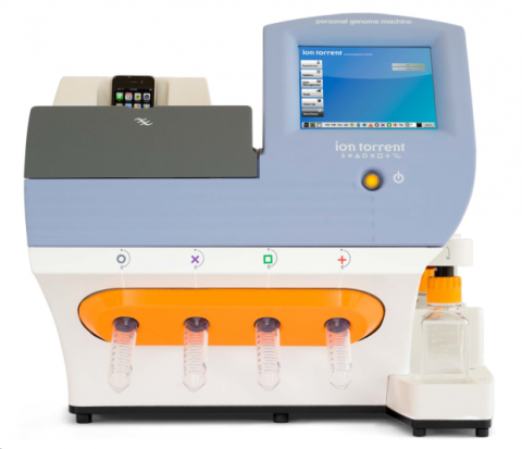
Ion Torrent sequencing
Ion Torrent sequencing works similarly to NGS technologies like pyrosequencing. However, instead of recording a visible light signal that results from a cascade of chemical reactions, Ion Torrent technology senses a hydrogen ion that is released naturally when a base is added to a DNA strand. An ion-sensitive layer detects these ions and records them as voltage spikes, which can be decoded into the original bases.
Assembling Aspects of Nextgen Sequencing
Sequence Alignment
In general, nextgen technologies result in very large numbers of reads that are shorter than those produced using capillary electrophoresis. Therefore, nextgen sequencing requires more robust algorithms to assemble the large quantity of data generated. Along with the increased output, the challenge is to manage and track sequence runs, and automating downstream data analyses. Several academic and private institutions provide core services for nextgen sequencing. Among them are Beckman Coulter Genomics, Massachusetts General Hospital, and the Office of Biotechnology at Iowa State University.
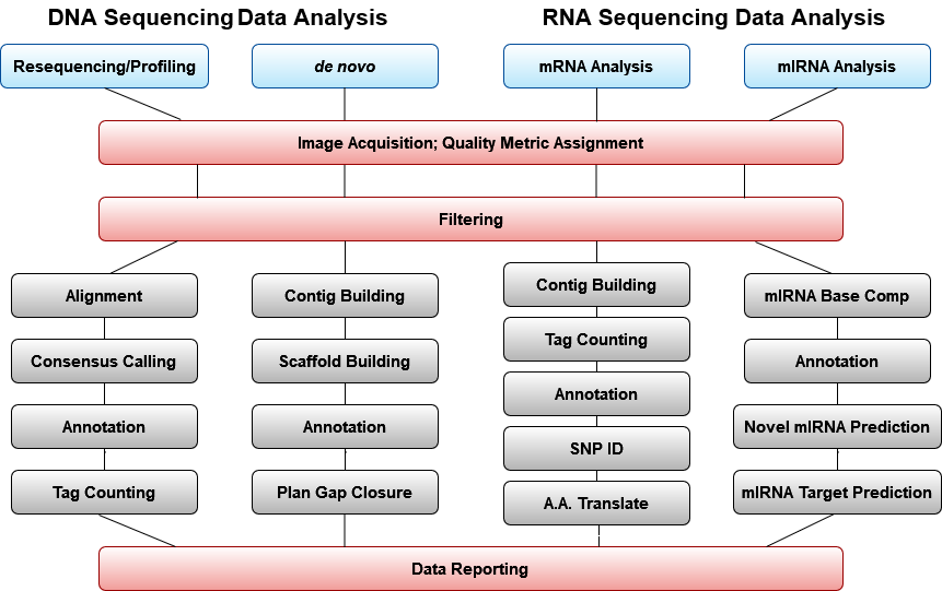
General Bioinformatics Workflow
Genotyping by Sequencing
Description
Next-generation sequencing has made it possible to sequence entire plant genomes in much shorter time and at a lower cost than using the approaches based on Sanger dideoxy sequencing (Glenn, 2011). Sequencing of multiple related genomes using NGS technologies can be done to sample genetic diversity within and between germplasm. However, even with NGS technologies, species with large complex genomes are a challenge to sequence. To address this challenge, genotyping-by-sequencing (GBS) was developed as a tool for association studies and genomics-assisted breeding for various crops species, including those with complex genomes.
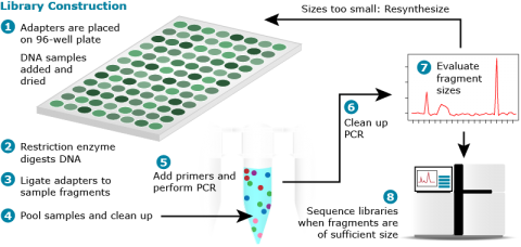
Library Construction
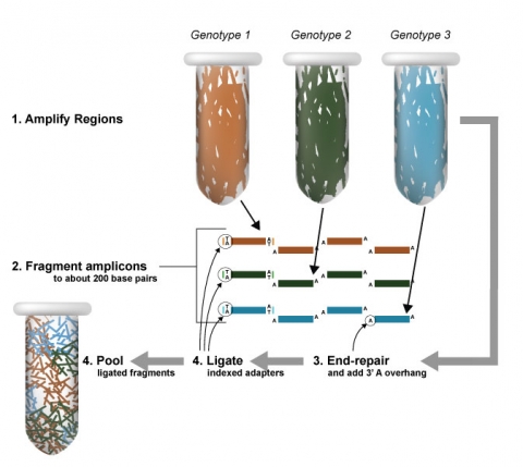
GBS uses restriction enzymes in combination with multiplex sequencing to reduce genome complexity sequencing cost (Fig. 4).
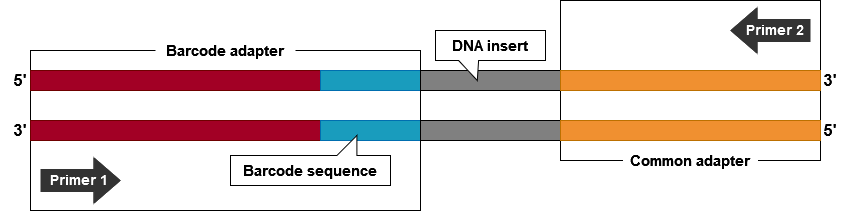
Sequence Barcoding
NGS technologies can produce more than 1 billion base pairs in a single sequencing run. A challenge is to use this enormous capacity for multiple DNA samples, for which only a fraction of the 1 billion bp sequence information is required. Barcoding enables to label sequences originating from a particular sample, and to pool barcoded DNA in a single sequencing run (Fig. 5). Barcodes in the context of DNA sequencing are short, unique sequences of DNA added to samples to be pooled, then processed and sequenced in parallel (Fig. 6). The sequence produced from the barcoded samples contains information to determine its origin. By barcoding the DNA, base-by-base error rate and array-to-array or day-to-day variability are reduced.
Adapter and Sequencing Primer Design
Multiplexed Sequencing Process
Sequence Barcoding
Haplotype Maps
Development of Haplotype Maps
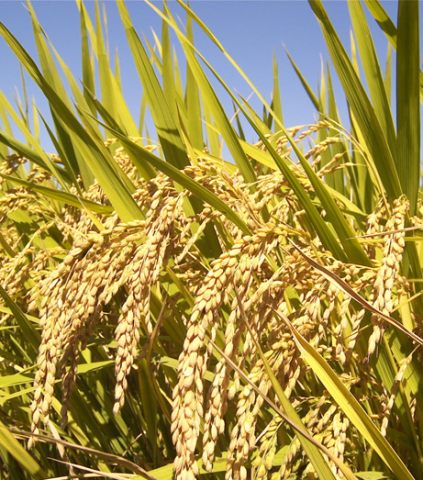
Genome-wide association studies (GWAS) require both phenotypic and genotypic data from multiple individuals. The concept of GWAS will be covered in the module “Cluster Analysis, Association and QTL Mapping”. Thus, GBS can be used to develop genotypic data for the construction of haplotype maps (HapMap) for GWAS. An example of the use of GBS for GWAS is from the work of Huang et al. (2010) describing the sequencing of 517 rice genomes using the Ilumina technology to generate about one-fold sequence coverage per genotype. The data generated by Huang et al. (2010) were used to construct a HapMap for GWAS for several agronomic traits in rice.
Data Imputation
The process of DNA sequencing is not free of error. Also, depending on the NGS system used, the length of base pair reads will be variable. Errors in sequencing and the length of the reads obtained by NGS may result in missing genotypes, thus affecting the quality of data.
The concern of missing data arises in almost all statistical analyses. This is actually what Huang and coworkers (Huang et al. 2010) encountered. Importantly, Huang and coworkers understood that linkage disequilibrium (LD) and the nonrandom correlation among allelic variants is extensive in rice. This meant that they could infer missing genotypes (missing data) with high confidence using data imputation (Marchini et al. 2007). Imputation is a statistical term describing substitution of a value for missing data.
The next section summarizes the approach used by Huang and coworkers to assign values to the missing genotypes.
Step 1: SNP Identification and Annotation
Single-base pair genotypes of 520 individuals obtained by Illumina sequencing were integrated to screen for single-nucleotide polymorphisms (SNPs) across the genome. Candidate SNPs were identified by comparing Illumina sequence data with the rice reference genome.
Step 2: Data Imputation To Assign Genotypes
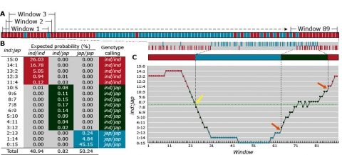
Sliding Window Approach
The sliding window (Fig. 8) is a multi-loci mapping algorithm commonly used in association mapping. It involves three steps: Local haplotypes are inferred from contiguous SNP loci Genotypes are grouped according to inferred haplotypes Statistics (F-test) for the genotype-phenotype associationand p-values are computed.
Map Construction by NGS Sequencing
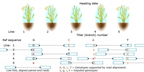
In Figure 9, variation in agronomic traits (e.g., heading date and tiller branch number) among lines are shown in the upper part of the figure. NGS sequences are aligned to the reference genome for genome-wide genotyping. Aligned reads (gray boxes) facilitate SNP (bases in upper case) identification among lines. Consistent patterns of mismatch between NGS sequence and the reference genome distinguish genetic variability from random sequence variation.
Bin Maps
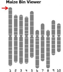
A bin (Gardiner et al. 1993) is a chromosome segment of about 20 cM flanked by two fixed core markers (a locus or probe that defines a bin boundary). A bin contains all loci within a left fixed core marker to the right fixed core marker. Assigning a locus to a bin is highly dependent on the precision of the mapping data, and increases in likelihood as the number of markers or mapping population increases in size. Bin maps contain coordinates named by the chromosome number, followed by a decimal, and a numeric identifier. 1.00 is the most distal (left or top-most, see arrow in Fig. 10) bin on the short arm of the chromosome. At right is the representation of bin boundaries for the 10 maize chromosomes.
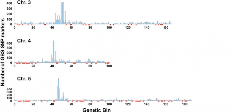
Bin Map Example
An example of application of GBS to develop a bin map for a crop with complex genome is provided from work by Poland et al. (2012). In this example, GBS was evaluated in wheat and barley, and a de novo genetic map was constructed using SNP markers from the GBS data (Fig. 11).
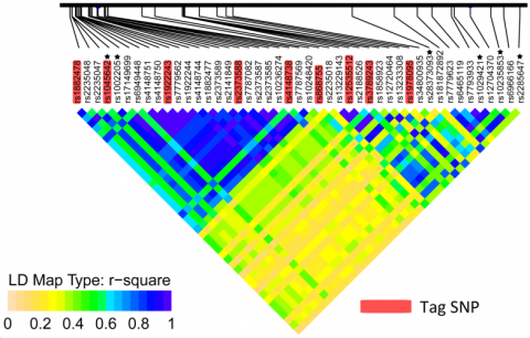
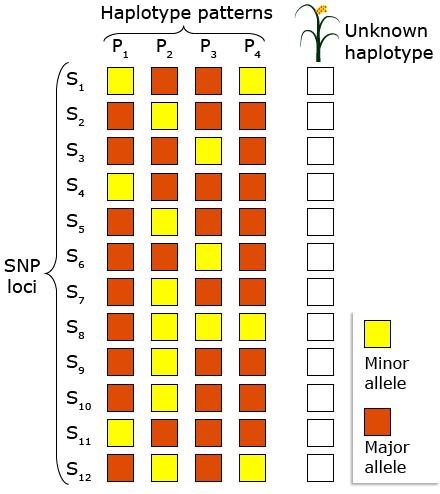
Tag SNPs
A tag SNP is a polymorphism in a region of the chromosome with high LD and can be used as a marker for genetic variation without genotyping an entire chromosome.
In the below figure, suppose SNPs in two alleles (major and minor) reveal a particular pattern among haplotypes.
DNA Markers
Development
The surge in the development of new tools for molecular genetics starting in the 1980s made it possible to identify genetic variation at the molecular level based on DNA changes and their impact on the phenotype. Such DNA changes (polymorphisms) can be exploited, e.g., as markers for a particular trait of interest, by plant breeders. Availability of an increasing amount of sequence data from sequencing projects together with new technologies such as next generation sequencing, and bioinformatic tools have reduced the cost of marker discovery and application.
Molecular Markers
Molecular or DNA markers reveal sites of variation in DNA. Variability in DNA facilitates the development of markers for mapping and detection or traits. Any DNA sequence can be genetically mapped, like genes leading to plant phenotypes. Prerequisite is, that there must be a polymorphism available for the sequence to be mapped, i.e., two or more different alleles. This can basically be a single nucleotide polymorphism (SNP), a single nucleotide variant at a particular position within the target sequence, or an insertion / deletion (INDEL) polymorphism. Target sequences can be amplified by various methods, including Polymerase chain reaction (PCR), and subsequently be visualized to generate “molecular phenotypes” comparable to visual phenotypes, that can be observed by using appropriate equipment. The main use of those SNPs and INDEL polymorphisms is as molecular markers. By genetic mapping as described above, linkage between genes affecting agronomic traits or morphological characters, and DNA-based SNP or INDEL markers can be established. It can be more effective in the context of plant breeding, to select indirectly for markers (DNA or non-DNA), than directly for target traits. Reasons can be: lower costs for marker analyses, the ability to run multiple such assays (for DNA markers) in parallel, the ability to select early and to discard undesirable genotypes or to perform selection before flowering, codominant inheritance of markers, among others. Below is a discussion on various types of markers used in plant breeding.
General Properties
DNA markers are readily detectable DNA sequences, whose inheritance can be monitored. The advantage of DNA-based markers is that they are independent of environmental factors. An ideal DNA marker (system) should possess the following properties:
- Be highly polymorphic
- Display co-dominant inheritance (to discriminate homozygotes from heterozygotes)
- Occur at high frequency in the genome
- Display selective neutral behavior
- Provide easy access
- Be simple to evaluate by available set of tools
- Display high reproducibility, and
- Facilitate easy exchange of data between laboratories
Historically, DNA markers can be grouped into three main categories: (1) hybridization-based markers, e.g. restriction fragment length polymorphism (RFLP) markers; (2) PCR-based markers, e.g., amplified fragment length polymorphism (AFLP), and simple sequence repeat (SSR); and (3) sequence or chip-based markers, e.g., some procedures for detecting single nucleotide polymorphism (SNP) markers. Examples of molecular markers belonging to the above three categories are further discussed.
RFLP
Restriction fragment length polymorphism (RFLP) markers involve cutting DNA into fragments and comparing patterns of variability in fragment size, or polymorphisms. RFLP patterns are analyzed by scoring an autoradiograph of a Southern blot. More information about RFLP is found in Crop Genetics eModule8.
Strengths of RFLP
- Co-dominance
- No sequence information is required
- Simplicity, not requiring costly instrumentation
- RFLP probe sequences can be used to develop additional markers e.g. Indel
- Transferability across related species
Weaknesses of RFLP
- Analysis requires large amounts of high quality DNA
- Low genotypic throughput (few loci detected per assay)
- Difficult to automate
- Use of radioactive probes restricts the analysis to specific laboratories
- Probes must be physically maintained not allowing sharing between laboratories
- Expensive
SSR
Simple Sequence Repeat (SSR) markers are widely used markers based upon the high rate of variation in microsatellite loci. SSRs represent a few to hundreds highly variable tandem copies of DNA repeats. Such tandem repeats of usually one to four bases are widespread in higher organisms. Many different microsatellite loci (>100,000) can be present in any plant species. SSRs are a result of slippage during DNA replication or unequal crossover during meiosis.
Variation in SSRs is observed by developing locus-specific primers that anneal to sequences flanking the repeat region; Polymerase Chain Reaction (PCR) is subsequently used to amplify the target region. Alleles (fragments) are visualized as bands with different migration pattern on a gel after electrophoresis. More recently, capillary electrophoresis is used, which also allows to multiplex up to about 16 SSRs per capillary.
The activity in the next screen will allow you to use database web tools to search for SSRs and design primers to detect SSR by PCR.
- Develop PCR primers to detect SSRs for maize teosinte branched1.
- Obtain Zea mays tb1 sequence from NCBI.
- Use the tb1 sequence you obtained from NCBI search for the tb1 locus in MaizeGDB.
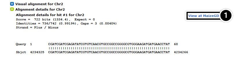
- In your BLAST results view the locations of tb1 in the maize genome.
- Select a hit with an E-value of 0.
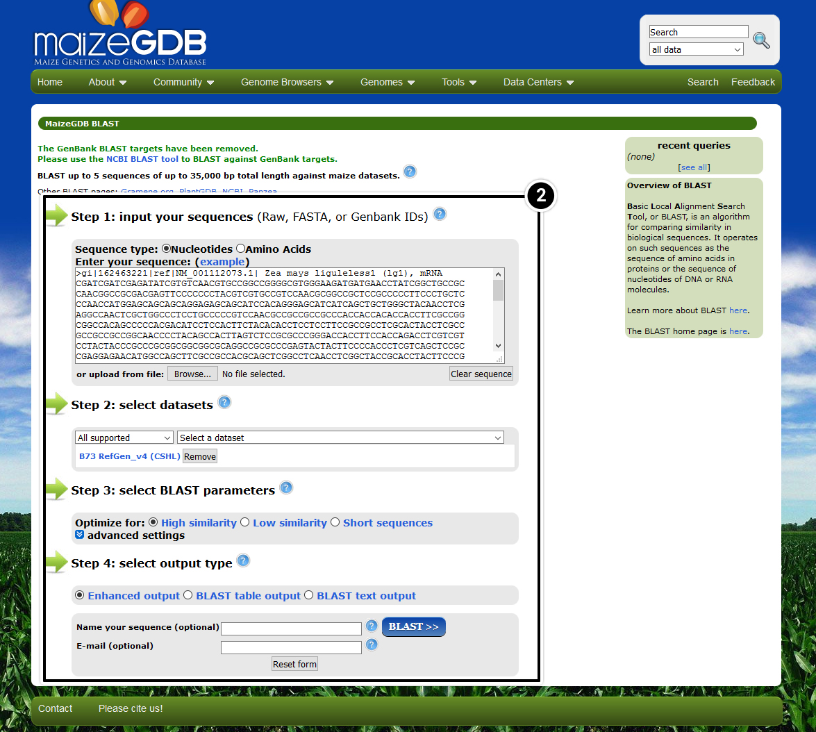
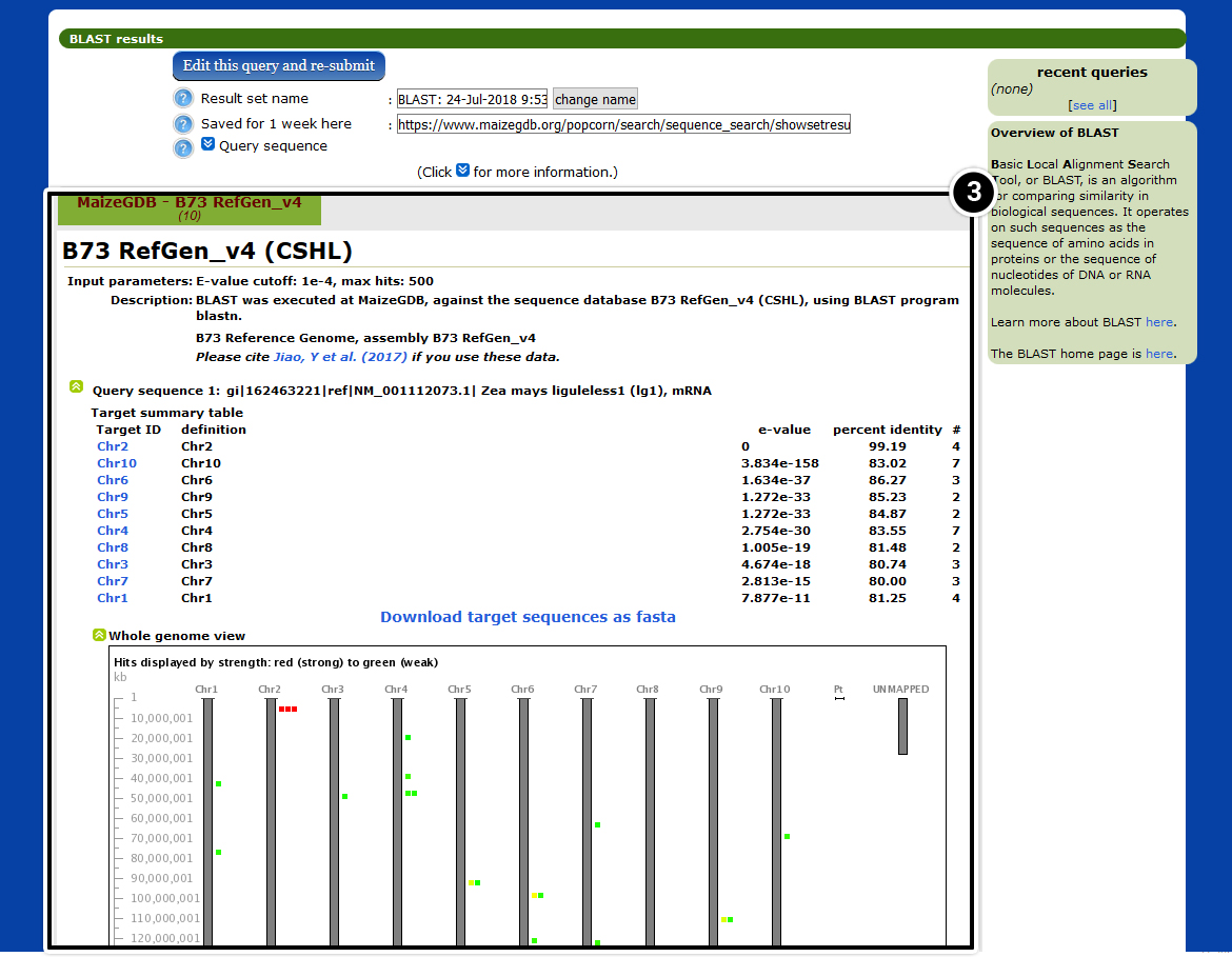
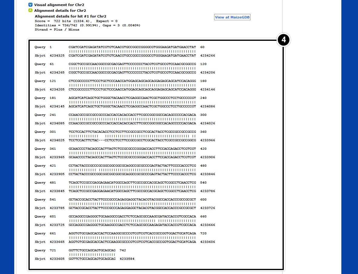
- Select View at Maize GDB
- Select Maize B73 RefGen_v2
- Select Download Decorated FASTA File
- Select Show 100 kbp to allow you to extract about 100 kbp containing the tb1 locus
- Select Go
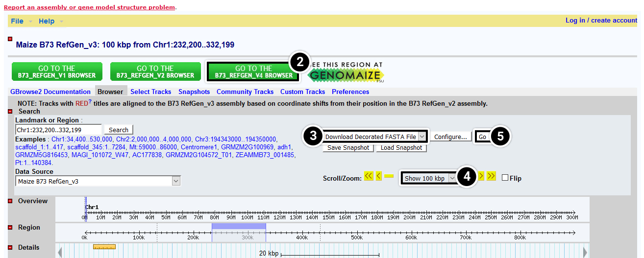
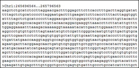
After performing the actions described in Step 5, a new window with the entire 100 kbp sequence you extracted will be displayed. Copy the sequence and proceed to step 6.
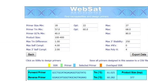
Several internet-based programs are available for searching microsatellites. For this exercise, you will use a web-based software called WebSat. To access WebSat, go to wsmartins.net/websat/.
- You have the option of pasting your copied FASTA sequence or uploading a FASTA file of your sequence. Also, you can change parameters related to the repeat.
- After entering the 100 kbp tb1 sequence, select Submit It!
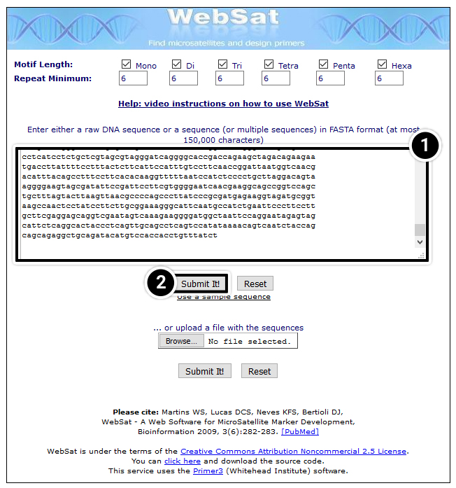
After submitting your sequence WebSat will search for SSRs within the sequence and return results with the option to design PCR primers. Design PCR primers around a repeat in the tb1 sequence by selecting a stretch of CTs found between positions 49,141 and 49,351.
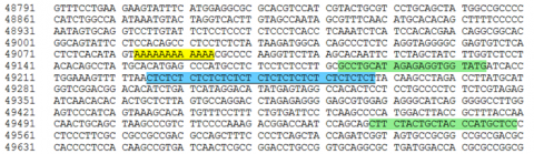
WebSat selects primers that fit the parameters of your choice to flank the SSR of your interest. In this case the forward and reverse primers around a stretch of CTs you selected will result in a PCR fragment of about 377 bp.
SSR – Strengths & Weaknesses
Strength of SSR markers:
- Hypervariable, multiple alleles (high PIC)
- In silico development straightforward
Weakness of SSR markers:
- Capability for multiplexing limited (max. 10-15)
- Affects costs/datapoint
- Few intragenic SSRs
More information online:
Transferability of molecular markers can help increase resolution of genomes that are not well characterized.
SSR markers located within genes can be used for direct selection of an allele.
AFLP
Amplified Fragment Length Polymorphism (AFLP) markers combine RFLP and PCR. In AFLP genomic DNA is digested with restriction enzymes followed a ligation step where adapters are added to both ends of the restriction fragments. PCR is carried out on the adapter-ligated mixture, using primers that target the adapter, but that vary in the base(s) at the 3’ end of the primer. Figures 21 and 22 in the text (see example of AFLP) describe the steps to detect and analyze AFLP markers.
Strength of AFLP markers:
- High marker index
- Amenable for automation
- Robust
- No prior sequence information required
- Special applications: Gene family profiling; Methylation assay
- Established service company: KeyGene
Weakness of AFLP markers:
- Random loci, might differ between populations
- Dominant marker system
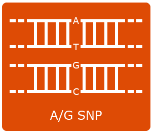
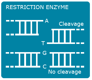
SNP
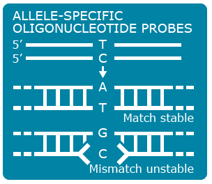
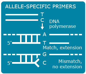
Single nucleotide polymorphisms (SNPs) are the most abundant kind of polymorphisms in eukaryotic genomes. SNPs are single nucleotide differences (transition or transversion) between allelic sequences. SNPs might cause polymorphisms detectable as RFLP or AFLP markers, if they occur in restriction enzyme recognition sites. Some principles exploited in SNP detection are shown in Figures 13, 14 , 15 and 16.
SNP Explanation
Overall, many different genotyping approaches are available ranging from low to high throughput. Some platforms permit users to pick custom SNPs but the highest throughput assays are available only in fixed contents. Not all custom SNPs will work for every format and multiple SNPs may be required to carry out most projects targeting specific SNPs. However, there are still trade-offs for throughput, that is, samples versus SNPs to be analyzed. Ultimately, cost will dictate how a SNP project is designed. Regardless of the study, design, quality control and tracking are critical to the success of the project. Laboratory Information Management Systems (LIMS) are important in every study design. The following are examples of SNP genotyping systems that are commonly used by plant breeders.
SNP: TaqMan Assays
TaqMan SNP assays (Fig. 17) are based on PCR using four oligonucleotide primers: (1) A set of forward and reverse primers that are designed and tested for each SNP, and (2) Two hydrolysis (Taqman) assay probes conjugated with fluorescent dyes and quenchers. Taqman probes are designed to anneal within a region of the PCR fragment resulting from the forward and reverse primers. The quencher ensures that a dye does not fluoresce before Taqman probes have annealed to their target during PCR. The PCR reaction is catalyzed by a polymerase enzyme with 5′ to 3′ exonuclease activity. The 5′ to 3′ exonuclease activity is required to cleave the quencher from the dye allowing fluorescence to be produced during PCR amplification.
An A to G transition is shown within the target DNA (DNA template).
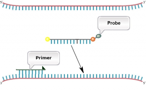
The 5′ to 3′ exonuclease activity of the polymerase degrades the probe that has annealed to the template. This releases the dye allowing fluorescence to occur.
SNP: Sequenom MassArray System
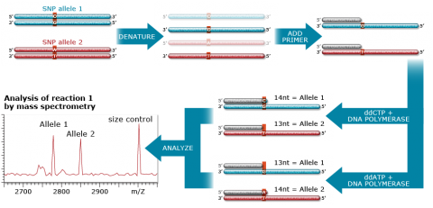
The Sequenom MassArray system (Fig. 18) uses highly multiplexed PCR reactions to screen multiple mutation sites simultaneously by primer extension combined with Matrix-Assisted Laser Desorption/Ionization-Timeof Flight mass spectrometry (MALDI-TOF-MS). Thesystem provides rapid and quantitative readout allowing detection of mutations, gene copy number, methylation status, and level of expression of allelic variants. Up to about 20 SNPs multiplied by about 400 samples can be analyzed at a time.
Key Steps in Sequenom MassArray System
SNP: Sequenom Massarray System
The three key steps in SNP analysis using the Sequenom system are (1) Target amplification (2) Primer extension and (3) Signal detection and ratio analysis. These steps are further described in Fig. 19.
SNP: GoldenGate Assay
The GoldenGate assay involves the addition of biotin to genomic DNA to immobilize the DNA on avidin-coated particles which bind biotin. The assay uses three oligonucleotide primers, two of these (P1 and P2) are specific for the two SNP alleles, and the third (P3) is a locus-specific primer that is tagged with a sequence for capture on solid support. In the reaction, the allele- and locus-specific primers anneal with the genomic DNA followed by extension using a DNA polymerase. After extension, the products are ligated to the tag sequence by a ligase. PCR primers containing fluorescence labels recognize the P1, P2, P3 sequences. The extension products containing the fluorescence labels are captured on the BeadArray containing complementary tag sequences for fluorescence detection.
Indels
Insertions and deletions (Indels) cause changes in DNA sequence by deletion or insertion. Indels can range in size from one or few bases to multiple megabases. Small deletions from a few base pairs to kilobases in length most often arise from unequal crossover during meiosis.
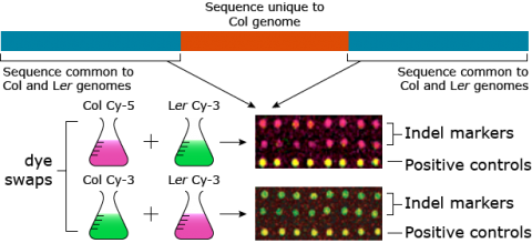
The Arabidopsis INDEL array (Salathia et al. 2007) is a microarray-based system (Fig. 20) that can be used to assess up to 240 polymorphic markers by hybridization. The array is based on 70-mer oligonucleotides of indels present in two Arabidopsis ecotypes, Columbia-0 (Col-0) and Landsberg erecta (Ler). PCR primers are also available for validation of array-based data. Groups of 16 lines can be genotyped together in a single experiment.
As shown in Figure 20, Salathia et al. (2007) swapped the dye labels for Col and Ler. What is the significance of dye swaps?
Basic Marker Applications
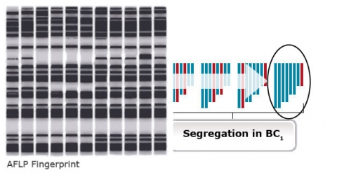
Marker Applications – Genetic Fingerprinting
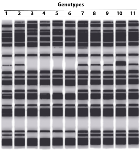
Genetic fingerprinting is a method that employs the uniqueness of DNA to classify individuals into distinct or similar groups. Based on the fact that genomes of different individuals will contain polymorphisms, a particular DNA profile can be established for a particular organism. This profile is specific to that individual and as unique as a fingerprint (Fig. 21).
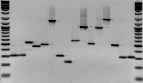
Genetic Fingerprinting by RFLP
The concept of fingerprinting is increasingly being applied to determine the ancestry of plants and animals. Genetic fingerprinting can be used in the breeding of endangered species or commercially important crops because it can help guarantee the authenticity of the plants. With the ability of obtaining highly specific DNA profiles, genetic fingerprinting can be used to protect from illegal use of patented or otherwise registered varieties. For commercially important crops that are difficult to characterize phenotypically, genetic fingerprinting is an important tool to identify genetic diversity within breeding populations. One of the earliest methods of genetic fingerprinting used hybridization-based RLFP markers. An example of genetic fingerprinting data is provided in Figure 22.
Genetic Fingerprinting Process
Genetic fingerprinting can be applied at all phases of cultivar development. The phases are described at right.
Phase 1: Identifying genetic variation
- In parent selection
- In recurrent selection
- In assigning individuals to heterotic pools
- In choosing genetic resources
Phase 2: Developing variety parents or testing hybrids
- To measure heterozygosity to predict hybrid performance
- In conducting backcrossing
Phase 3: Seed multiplication and variety protection
- To ensure purity of hybrids and blends
- For variety approval
- To identify “essentially derived varieties” (EDV)
Gene Tagging
If markers flank a gene of interest, the likelihood of a recombination event occurring between markers and gene of interest depends on the genetic distance between them. Thus, the closer the marker is to the gene controlling a trait of interest, the higher chance that there will be no recombination between gene and marker. Absolutely linked markers co-segregate with the trait of interest.
A marker linked to a gene controlling a gene of interest can serve as a “tag” for that gene/trait (Fig. 23).
Use of Linked Markers: Step 1
Use of Linked Markers and Fingerprinting to Assist Backcrossing
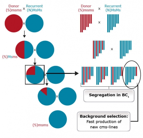
Marker-assisted backcrossing involves three steps (Figs. 24-26):
Step 1. Selection of donor allele at the markers linked to target gene to reduce loss of target allele due to recombination. In this step, markers are useful if the trait is controlled by a recessive allele, or when multiple resistance genes are to be obtained from the donor. Also, markers are useful for environmentally-sensitive genes and for expensive phenotypes, for example, grain quality.
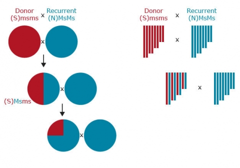
Step 2. Selection of recurrent parent allele at other linked markers. This helps reduce linkage drag when introgressing wild or exotic germplasm.
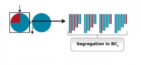
Step 3. Selection of recurrent parent allele at unlinked markers throughout the genome (background selection). It is all a matter of probability to identify backross progeny that are similar to the recurrent parent (Fig. 26). Therefore, markers inherent to the recurrent parent (background markers) can help identify progeny most similar to the recurrent parent.
Use of Linked Markers: Step 2
Step 2. Selection of recurrent parent allele at other linked markers. This helps reduce linkage drag when introgressing wild or exotic germplasm.
Use of Linked Markers: Step 3
Step 3. Selection of recurrent parent allele at unlinked markers throughout the genome (background selection). It is all a matter of probability to identify backross progeny that are similar to the recurrent parent (Fig. 27). Therefore, markers inherent to the recurrent parent (background markers) can help identify progeny most similar to the recurrent parent.
Markers and Selection
Use of Linked Markers and Fingerprinting to Assist Backcrossing
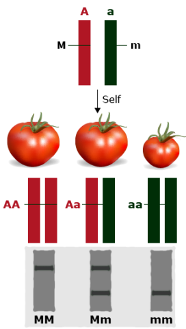
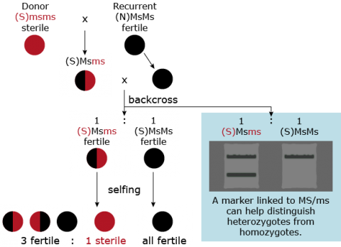
Markers are useful for foreground selection of lines having the donor allele in heterozygous condition. An example of the use of markers for foreground selection is described in Figure 27. Without a marker it would not be possible to distinguish progeny heterozygous for the male sterility trait (Msms) from homozygous (MsMs) genotypes because both scenarios result in fertile plants. The use of a co-dominant marker linked to Ms/ms, heterozygotes helps identify heterozygotes and eliminates the need to expend time and resources for selfing and scoring individuals based on pollen production.
DNA Versus Non-DNA Markers
Groups of Non-DNA Markers
Genetic markers are broadly classified into two groups. (1) DNA markers: those based on detection of DNA. (2) Non-DNA markers: those based on visually distinguishable traits, also referred to as morphological markers (e.g. flower color or seed shape); and those based on gene products, referred to as biochemical markers (e.g. RNA, protein, and other cellular metabolites).
The advantage of DNA markers is that they are not affected by environmental factors. However, presence of a particular DNA sequence may not always lead to the expected expression for a trait of interest. This is, because the expression of a particular allele depends on environmental conditions, and also interaction with other genes. Thus, even though an allele with a known effect on a particular trait is present, it might not result in the expected phenotype. Therefore, DNA markers are considered to be a measure of the genetic potential of an individual. The equivalent in human genetics is the risk concept. Based on DNA information, it is possible to predict the risk of a patient for showing a particular condition (e.g., 30% to get pancreatic cancer at a certain age). However, whether this condition is expressed, depends on other circumstances. In contrast, if RNA- or metabolite-based biomarkers for this cancer type are available, onset of this condition can be predicted with high accuracy. Thus, non-DNA markers are indicative of the realized potential of an individual.
Visible Markers
The advantage of morphological markers, also called visible markers, is that they are in general easy to score. However, morphological markers are affected by environmental conditions, making their use less reliable across environments. Also, morphological markers are limited in number compared to the abundance of DNA markers. Biochemical markers are affected by the developmental stage of the plant, and the cell type from which they are isolated. This has to be carefully selected. This is a major difference compared to DNA-markers, which are stable and valid, independent of the tissue from which the respective DNA has been isolated. The World Health Organization defines a biomarker as any parameter that can be used to measure an interaction between a biological system and an environmental agent, which may be chemical, physical or biological. Therefore, diagnosis of presence of disease condition and possible treatment requires use of biomarkers. In conclusion, the term biomarker is broadly defined and may include DNA- and non-DNA markers. However, sometimes the term biomarker is used in a more narrow sense for biochemichal non-DNA markers.
Genetic Pathways from DNA to RNA
To understand the relationship between DNA markers and non-DNA markers, review the pathways by which genetic information in deoxyribonucleic acid (DNA) is transferred to ribonucleic acid (RNA) molecules (called transcription), and then transferred from RNA to a protein (termed translation) by a code that specifies the amino acid sequence. Epigenetic mechanisms including DNA methylation/ demethylation and histone acetylation/deacetylation may also impact gene expression (Fig. 28).
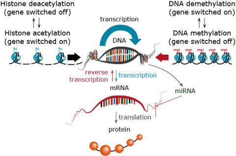
Figure 28 illustrates two steps in gene expression, transcription (production of mRNA from DNA), and translation (production of proteins from mRNA). Not all genes produce mRNA that can be translated into proteins. Certain genes are transcribed into non-coding RNAs (e.g. micro-RNAs – miRNAs) or short-interfering RNAs – siRNAs) that serve a regulatory function during plant growth and development. A gene can be either “on” or “off” depending on the cell-type, stage of development, and environmental signals, meaning that at any moment each cell makes coding and non-coding RNA from only a proportion of its genome.
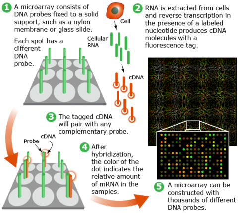
Microarray Technologies
Development of a microarray starts with the synthesis of probes. Probes can be either (a) cDNA sequences derived from expressed sequence tags (EST) clones or small fragments from PCR or (b) synthetic oligonucleotides, short sequences designed to complement genomic targets of interest. The oligonucleotides may be long (60-mer) or short (25-mer) depending on the purpose of the experiment. Longer probes bind their targets with higher specificity than shorter probes. However, shorter probes may be spotted at a higher density on an array than longer probes, thus reducing the cost of array production.
Microarray technologies allow parallel assessment of thousands of genes in a single experiment to generate data for gene function, or trait characterization. Microarray analysis involves hybridization of target sequences with gene-specific probes spotted on an array (Fig. 29) For the development of RNA-based markers, target sequences are prepared from total RNA or mRNA.
Microarray Analysis (1)
Micro RNAs (miRNAs) are small non-coding RNAs which play key roles in regulating the translation and degradation of mRNAs. Genetic or epigentic alterations may affect miRNA expression, thereby leading to aberrant target gene(s) expression in diseases such as cancer. Thus, miRNAs may also provide useful biomarkers for diseases diagnosis. For example, a study by Yanaihara et al. (2006) identified 43 miRNAs that are uniquely expressed in affected lung tissue. Recent studies indicate that miRNAs expression in plants is affected by stress conditions such as drought (Li et al. 2011).
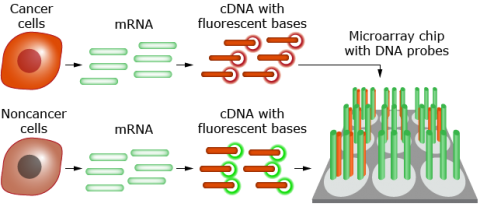
The differences in mRNA profiles between genotypes can be exploited to develop biomarkers for predicting future performance of an individual. In humans, for example, variation in gene expression can be used to predict the occurrence of cancer (Fig. 30).
- Cancer and noncancer cells are removed from patients with breast cancer.
- Messenger RNA from the cells is converted to cDNA and labeled with red (cancer cells) or green (noncancer cells) fluorescent nucleotides.
- The cDNAs are mixed and hybridized to DNA probes on a chip.
- The chip is scanned spot by spot.
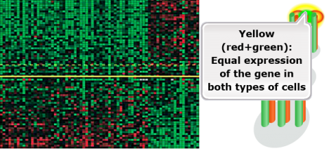
- Each spot represents the expression of one gene in one patient’s tumor compared with the expression of that gene in her noncancer cells.
- Tumors above the yellow line came primarily from patients who remained cancer-free for at least 5 years.
- Tumors below the yellow line came primarily from patients in whom the cancer spread within 5 years.
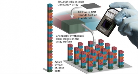
Microarray Analysis (2)
1. On-slide synthesized arrays Such arrays are prepared by chemical synthesis of probes on the array surface, e.g., Affymetrix arrays (Fig. 31).
Microarray Analysis (3)
- On-slide synthesized arrays Such arrays are prepared by chemical synthesis of probes on the array surface, e.g., Affymetrix arrays.
Microarray Analysis (4)
- Spotted cDNA arrays This type of arrays is prepared by spotting purified PCR products from a cDNA library on glass using a robotic arrayer.
- Spotted gene-specific sequence tag arrays Similar to spotted cDNA arrays, PCR products are spotted on glass by a robotic arrayer. However, in contrast to spotted cDNA arrays, spotted gene-specific sequence tags are developed by PCR using primers targeting unique segments of genes or BAC clones.
- Spotted long oligonucleotide arrays These arrays constitute oligos ranging from 50-70 base chemically synthesized to match a particular region of a gene of interest. The 50-70mer oligos are spotted on glass slides robotically.
Protein-Based Markers
Common protein markers are isozymes. Isozymes are enzymes with similar function derived from more than one locus. Isozymes are encoded by gene families resulting from duplication events. Isozymes are different from allozymes in that allozymes represent one enzyme derived from a single locus.
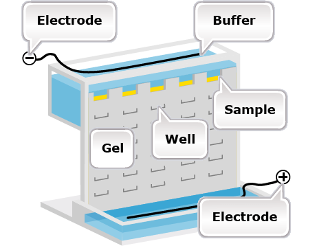
Isozymes are analyzed by a procedure called electrophoresis. Electrophoresis is a technique for separating macromolecules on a gel by means of an electric field and specific chemical staining (Fig. 33). Therefore, to be useful as markers, isozymes must be electrophoretically resolvable (i.e., bands can be clearly separated for visualization on a gel), and detectable by various in-gel assay methods.
Isozymes
The advantage of isozymes is that they are robust and highly reproducible. Also, isozymes have codominant expression, meaning that both homozygotes can be distinguished from the heterozygote and neither allele is recessive. However isozymes are gene products, so they reveal only a small subset of the actual variation in DNA sequences between individuals and do not reveal variation in the non-coding regions of the genome. Other limitations of isozymes as markers include: (i) data complexity as a result of dimers or multimers of the enzymes; (ii) multi-allelic and multi-locus systems can make interpretation of the banding patterns difficult; (iii) the system is limited to those enzymes that can be detected in situ, resulting in a narrow coverage of the genome; (iv) relatively few biochemical assays are available to detect isozymes; and (v) the assay is based on a phenotype, and thus sensitive to the environment.
Currently, isozymes are used mainly for germplasm identification and population genetics studies. Other examples of application of proteomic approaches are listed below.
- Two-dimensional polyacrylamide gel electrophoresis was used to detect polymorphic protein markers in several plant species (Vienne et al. 1996).
- A proteomic approach was used to identify protein markers in lung cancer (Mehan et al. 2012).
- Isozymes were useful in developing the linkage map for tomato (Bernatzky and Tanksley, 1986).
- Maquet et al. (1997) used allozyme markers to study the genetic structure of Lima bean (Phaseolus lunatus L.) base collection.
- Ibáñez et al. (1999) evaluated isozyme uniformity in a wild extinct insular plant [Lysimachia minoricensis J.J. Rodr. (Primulaceae)].
- Rouamba et al. (2001) assessed allozyme variation of onion (Allium cepa L.) populations from West Africa.
Metabolite-Based Biomarkers
As described earlier, in human health, changes from healthy states to disease state and conditions can be described in terms of important metabolites of cells. A similar approach can be used to determine biomarker metabolites in plants during growth and development. For example, a study by Tarpley et al. (2005) established a biomarker metabolite set for rice during development.
The advantage of metabolite-based markers is that their levels are more closely associated with phenotypes than DNA markers. Therefore, establishing a set of metabolite biomarkers for a plant may be useful in predicting agronomic performance under different environments (Sulpice et al. 2009, 2010; Steinfath et al. 2010).
Techniques for Profiling
Two techniques used largely for profiling metabolite biomarkers are: (1) mass spectrometry (MS); and (2) nuclear magnetic resonance (NMR). Examples of methods for establishing metabolite biomarkers in plants include gas chromatography- mass spectrometry (GC-MS), liquid chromatography mass-spectrometry (LC-MS), and NMR. The application of some of these methods is described in the work by Skogerson et al. (2009) to establish metabolite profiles for various wines as biomarkers for wine sensory properties. The advantage of such wine biomarkers is that they may be used to replace expensive and laborious sensory panels (Skogerson et al. 2009). Also, such biomarkers may be useful for various regulatory purposes, for example, detection of adulterations.
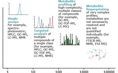
In evaluating biomarkers, there is a trade-off between metabolic coverage and the quality of the metabolite data. As shown in Figure 34, analysis of a single metabolite or a metabolite class yields data of higher quality than broad analysis for several chemical classes.
Plant Phenomics
Plant phenomics is the study of how genetic makeup of an individual influences its physical and biochemical characteristics in a particular environment (Furbank and Tester, 2011). High-throughput phenomics facilities are using automated plant imaging for the repeated, non-destructive acquisition of high-dimensional phenotypic data on a whole-plant scale.
For example, The Australian Plant Phenomics Facility uses the Plant Accelerator. The LemnaTec phenomics systems can handle small plants (Arabidopis) and large plants (corn) to measure various parameters including, leaf area, chlorophyll content, stem diameter, height, biomass, color, and leaf tracking over time. The LemnaTec technology can also be used to measure responses to salt, and drought stress. The application of phenomics is important for studying complex stress traits such as drought because non-destructive imaging methods allow temporal resolution and monitoring of the same plants during the experiment (Berger et al. 2010).
Ultimately, phenomic data (e.g., canopy reflectance) can be used as indirect trait for agronomic traits of interest. An example is the measurement of canopy “greenness” to describe the nitrogen use efficiency (NUE) of plant genotypes.
References
Akhunov, E., C. Nicolet, and J. Dvorak. 2009. Single nucleotide polymorphism genotyping in polyploidy wheat with the Illumina GoldenGate assay. Theor Appl Genet 119:507-517.
Baskin et al. 2009. http://www.geospiza.com/Products/WhitePaper_06102009.pdf
Clark, R.M. 2010. Genome-wide association studies coming of age in rice. Nature Genetics 42:11, 926-927.
Craig, D.W., et al. 2008. Identification of genetic variants using bar-coded multiplexed sequencing. Nature Methods 5, 887-893. doi:10.1038/nmeth.1251
DiGuistini et al. 2009. De novo genome sequence assembly of a filamentous fungus using Sanger, 454 and Illumina sequence data. Genome Biology 10:R94.
Eid et al. 2009. Real-Time DNA sequencing from single polymerase molecules. Science 323: 133-138.
Elshire et al. 2011. PLoS ONE 6. doi:10.1371/journal.pone.0019379
Fernie et al. 2004. Metabolite profiling: from diagnostics to systems biology. Nature Reviews Molecular Cell Biology 5, 763-769 (September 2004). doi:10.1038/nrm1451
Flicek, P., and E. Birney. 2009. Sense from sequence reads: methods for alignment and assembly. Nature methods. 6:S6-S12.
Hawkins et al. 2010. Next-generation genomics: an integrative approach. Nature Reviews Genetics. 11:476-486.
Huang et al. 2009. High-throughput genotyping by whole-genome resequencing. Genome Res. 2009 Jun;19(6):1068-76. doi: 10.1101/gr.089516.108
Illumina, Inc. 2006. GoldenGate Assay workflow. https://www.illumina.com/documents/products/workflows/workflow_goldengate_assay.pdf
Li, H., and N. Homer. 2010. A survey of sequence alignment algorithms for next-generation sequenc-ing. Briefings in Bioinformatics. 11: 473-483.
MaizeGDB. Maize bin viewer. http://www.maizegdb.org/bin_viewer
Maxam, A M., and W. Gilbert. 1977. A new method for sequencing DNA. Proc. Natl. Acad, Sci. USA. 74:560-564.
Metzker. 2010. Sequencing technologies — the next generation. Nature Reviews Genetics. 11:31-46
Munroe, D., and T. J. R. Harris. 2010. Third-generation sequencing fireworks at Marco Island. Nat. Biotechnol. 28:426-428.
Perkel, J. 2008. SNP genotyping: six technologies that keyed a revolution. Nature Methods 5:447-454.
Poland, J.A., P.J. Brown, M.E. Sorrells, and J-L Jannink. 2012. Development of High-Density Genetic Maps for Barley and Wheat Using a Novel Two-Enzyme Genotyping-by-Sequencing Approach. PLoS ONE 7(2): e32253. doi:10.1371/journal.pone.0032253
Rothberg et al. 2011. An integrated semiconductor device enabling non-optical genome sequencing. Nature. 475:348-352.
Salathia, N., H. N. Lee, T. A. Sangster, et al. 2007. Indel arrays: an affordable alternative for genotyping. Plant J. 51: 727-737.
Schneeberger et al. 2009. SHOREmap: simultaneous mapping and mutation identification by deep sequencing. Nat Methods. 6:550-551.
Schneeberger, K., and D. Weigel. 2011. Fast-forward genetics enabled by new sequencing technologies. Trends Plant Sci. 16:282-8.
Shendure, J., and H. Ji. 2008. Next-generation DNA sequencing. Nature Biotechnology 26:1135-1145.
Syvänen, A. 2001. Accessing genetic variation: genotyping single nucleotide polymorphisms. Nat Rev Genet. 2:930-942.
Syvänen, A. 2005. Toward genome-wide SNP genotyping. Nat Genet. 37: S5-S10.
ThermoFisher Scientific. Contract Research Organizations To Adopt Ion Torrent Next-Generation Sequencing Platform. http://news.thermofisher.com/press-release/life-technologies/contract-research-organizations-adopt-ion-torrent-next-generation–0
Xu, Y. Molecular Plant Breeding. CABI, Wallingford, Oxon.
A genetic change in a population or species over time.
One of the building blocks of DNA or RNA, each of which contains a nitrogenous base attached to a five-carbon sugar that in turn is attached to one or more phosphate groups.
The phenotypic and genotypic differences among individuals in a population.
(1) The process by which organisms change over time.
(2) The genetic change in a population or species over time.
An identifiable segment of DNA (e.g., RFLP, VNTR, microsatellite) with enough variation between individuals that its inheritance and co-inheritance with alleles of a given gene can be traced; used in linkage analysis.
A population that has more than one common allele present at a locus.
the reproductive or vegetative propagating material of the following categories of plants: (i) cultivated varieties (cultivars) in current use and newly developed varieties; (ii) obsolete cultivars; (iii) primitive cultivars (landraces); (iv) wild and weed species, near relatives of cultivated varieties; and (v) special genetic stocks (including elite and current breeder's lines and mutants)
(1) All of the genes shared by individuals in a group of interbreeding individuals.
(2) In plant genetic resources, use is made of the terms 'primary', 'secondary' and 'tertiary' gene pools. In general, members of the primary gene pool are inter-fertile; those of the secondary can be crossed with those in the primary gene pool under special circumstances; but to introgress variation from the tertiary gene pool, special techniques are required to achieve crossing.
The use of in vitro techniques to produce DNA molecules containing novel combinations of genes or other sequences in living cells that make them capable of producing new substances or performing new functions.
Usage: A popular term for such technologies as a whole.
The fusion of plant protoplasts derived from somatic cells that differ genetically
A general term used to describe the culture of cells, tissues or organs in a nutrient medium under sterile conditions
A genotype formed when haploid cells undergo chromosome doubling.
A genotype containing more than two paired sets of chromosomes
A collection of specific alleles (particular DNA sequences) in a cluster of tightly-linked genes on a chromosome that are likely to be inherited together.
the occurrence of some combinations of alleles or genetic markers in a population more often or less often than would be expected from a random formation of haplotypes from alleles based on their frequencies.
a DNA sequence variation occurring commonly within a population (e.g. 1%) in which a single nucleotide — A, T, C or G — in the genome (or other shared sequence) differs between members of a biological species or paired chromosomes.
Construction of a localized (around a gene) or broad-based (whole genome) genetic map to determine the location of a locus (gene or genetic marker) on a chromosome.
A double-stranded, helical, structure comprised of base pairs (ATCG) that carry genetic information in the nucleotide sequence. It is normally found, packaged or condensed, within the chromosomes that reside within the cell’s nucleus. Single-stranded DNA is unstable and rarely found in nature.
A single-stranded, linear structure comprised of base pairs (UAGC ) that carry genetic information in the nucleotide sequence. It is used during replication to copy the DNA sequence and is known as mRNA once it's outside the the nuclear membrane. Transfer RNA (tRNA) is used during translation at the ribosome, as amino acids (AA's) are linked together. The long string amino acids form a polypeptide that is later folded into a functional protein.
Two or more enzymes capable of catalyzing the same reaction but differing slightly in their structures and consequently in their efficiencies under various environmental conditions.
A genetic marker in which the heterozygotes can be distinguished from the homozygotes.
