
Chapter 6: Marker Assisted Backcrossing
Thomas Lübberstedt; William Beavis; and Walter Suza
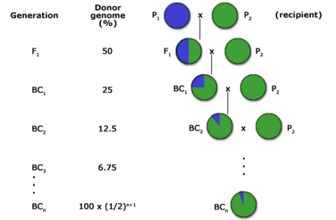
Backcrossing (BC) describes a plant breeding procedure used to incorporate one or several genes into an adapted or elite variety. The BC method (Fig. 1) is a form of recurrent hybridization by which a superior characteristic is added to an otherwise desirable genetic background. In this method the breeder has considerable control of the genetic variation in the segregating population in which the selections are to be made.
- Understand backcross (BC) breeding
- Understand the main application of molecular markers for BC breeding
- Understand factors influencing the efficiency of BC breeding
General Considerations
The Goal of Backcrossing
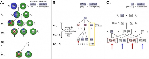
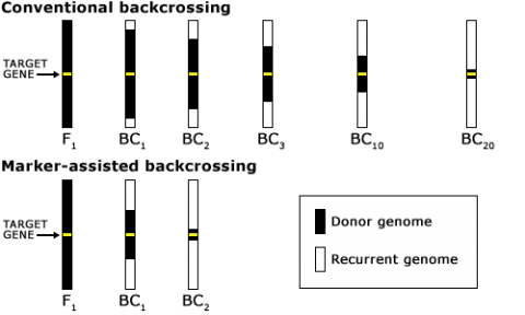
The goal of a BC program is to recover a pure line or inbred that will contain the novel allele and be as good as the recurrent parent for all other important traits. For this reason, the BC method has been extensively used for transferring alleles for novel traits into elite germplasm (Fig. 2). The novel alleles may be natural mutations or may be the result of mutagenesis or genetic engineering.
Genotype Structures
Backcross works well when a variety to be improved is an inbred line. Also, the inheritance of the trait to be introgressed must be monogenically or oligogenically inherited for backcross to work. The method does not work (well) for clonal and synthetic cultivars because self-pollination or the mating of related individuals does not (fully) recover the recurrent parent which thus is in conflict with the goal of the BC method: to add one or few genes to the recurrent parent. The desired trait for backcrossing must be present in a donor genotype which can be crossed with the cultivar to be improved. Thus, the trait must be available in the primary or secondary germplasm pool.
The expected proportion of genome originating from the recurrent parent in backcross generations can be estimated using the following formula:
[latex]E_t \approx 1-(\frac{1}{2})^{t+1}[/latex]
where:
Et = expected proportion of the recurrent parent genome
t = backcross generation
Limitation of BC Method
The goal of the BC method for line and hybrid breeding is to add one or few genes to an existing line or variety. However, varieties in major crops have a short half-life, maybe only a couple of years. Thus, until the gene(s) have been introduced into an existing variety, it might already be outdated. The challenge for breeders is, to introduce genes of interest (including transgenes) into the most recent germplasm, which increases the effort. A recent study using computer simulation suggests incorporating intercrossing in trait introgression might be more efficient in lowering the cost and time than the BC method (Zheng et al. 2023).
Marker-Assisted Backcrossing
Examples of Marker-Assisted Backcrossing
As mentioned above, five to eight BC generations are usually required for gene introgression into a target variety. However, this consideration is also affected by the following factors:
- Genetic similarity between donor and recipient
- Necessity to recover the properties of the recipient
- Linkage between undesired genes of the donor and the target gene, referred to as “linkage drag” MABC is widely applied in plant breeding programs (Collard and Mackill, 2008).
3 Steps of MABC
In general, MABC Involves Three Steps:
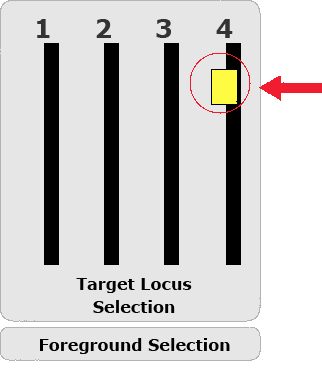
Step 1: Foreground selection for the target gene(s). Marker-based foreground selection is particularly useful, if the target gene is recessive, or for combining redundantly acting target genes. Also, foreground selection is useful for environmentally-sensitive genes and in case of expensive phenotyping, for example, some grain quality traits. Finally, marker-based foreground selection enables early selection and elimination of undesirable plants, thus reducing costs related to growing and managing plants.
Step 2: Background selection near the target gene(s) to reduce linkage drag when introgressing wild or exotic germplasm.
Step 3: Background selection throughout the genome. Markers enable the identification of progeny most similar to the recurrent parent. Thus, the use of markers helps accelerate a BC program.
Parameters to be optimized in MABC:
- Optimal distance between target locus and flanking markers for a given population size
- Minimal number of individuals for detecting recombinants in a given marker interval
- Minimal number of data points to achieve fast completion of BC program
- Allocation of marker analyses to different BC generations
Foreground Selection
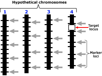
Marker-assisted foreground selection involves the use of markers closely linked to the target gene as diagnostic tools (Fig. 3) for genes controlling traits that are difficult to evaluate, such as recessive traits, or traits that express late during plant development. Ideally, a marker derived from the target locus can be used for foreground selection. More information about foreground selection can be found here:
Estimating the Number of Individuals Required for Foreground Selection
It is important to estimate the minimum number (n) of individuals that are required for successful foreground selection for g unlinked target genes, in case gene-derived markers are available for all target genes.
The minimum population size required to find with probability q = 0.99 at least one BC1 individual of Type 2 can be estimated by the following binomial expression:
[latex]q = (_{m}^{n}) p_{i}^{m} (1-p_i)^{n-m}[/latex]
where:
m = number of individuals with target genotype
n = minimum sample size
q = probability to find at least one individual of a desired genotype
p = probability for occurrence of a particular genotype i
The probability q that at least one individual among n individuals has the desired genotype (Also, see Lubberstedt and Frei, 2012) is:
[latex]q = P \left \lfloor m > 0 \right \rfloor = 1 - P \left \lfloor m = 0 \right \rfloor = 1 - (1-p)^n[/latex]
From the above equation, the minimum population size needed to identify at least one desired genotype in the population can be derived from the following equation:
[latex]n \geq \dfrac{ln (1-q)}{ln (1-p)}[/latex]
Estimating Number of Genes to Consider
The probability p that a BC individual has the desired genotype when g genes are under consideration is calculated using the following formula:
[latex]p = (\frac{1}{2})^g[/latex]
The probability of finding a BC individual with the desired genotype diminishes with an increasing number of genes to be introgressed. Therefore, MABC is most efficient for introgression of one or fewer target genes.
Trait Introgression
Trait introgression is one of the important examples for foreground selection. In that case, the target gene is known. Thus, a marker derived from the target gene can be derived. A suitable marker for use in foreground selection should possess the following properties:
- Co-dominant inheritance to allow distinction between homozygotes and heterozygotes. Co-dominant markers are most useful for marker-assisted backcrossing because selection among backcross progeny involves selection for heterozygous progeny. If a dominant marker, such as an AFLP band, is used for selection, it will be informative during backcross generations, if the dominant allele (conferring band presence) is linked to the donor parent allele. If the recessive allele (conferring band absence) is linked to the donor parent allele, then all backcross progeny will either be heterozygous or homozygous for the dominant allele that produces the marker band, so the marker will be useless for selection among backcross progeny
- Reproducible
- Allows automation for high-throughput scale
- Linked with target gene(s) of interest
During foreground selection, there is a risk that the target gene is lost due to recombination between target gene and flanking marker(s) used for foreground selection. To determine the probability that a desired allele will be lost during backcrossing, let us use the following model.
Probability Model
Assume there are two marker alleles m1 and m2, and two alleles of the target gene a1 and a2 (r = recombination rate between m and a). m1 is linked in coupling with a1 and in repulsion with a2. The goal is to backcross a2 into our elite line, which contains a1. At the F1 generation the backcross progeny will be of the following genotype:

| Gamete | Frequency |
|---|---|
| m1 a1 | ½(1 – r) |
| m1 a2 | ½(r) |
| m2 a1 | ½(r) |
| m2 a2 | ½(1 – r) |
and will produce gametes listed in Table 2.
| Genotype | Frequency |
|---|---|
| m1m1a1a1 | ½(1 – r) |
| m1m1a1a2 | ½(r) |
| m1m2a1a1 | ½(r) |
| m1m2a1a2 | ½(1 – r) |
The objective is to select the a1a2 plants in the BC1F1 generation by selecting for the m1m2 plants. However, there is a probability that the target allele may be lost in the m1m2 plants due to recombination (r). The probability (P) to lose the allele (by selecting an individual of the a1a1 genotype) is:
[latex]P(m1m2a1a1) = (2)r/(2) = r[/latex]
The Reliability of Selection
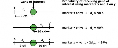
Thus, if the recombination frequency (r) between flanking markers and gene loci is 5%, the chance of selecting a plant that is m1m2 but does not have the target gene (a2) is also 5%. Therefore, it is critical to use markers that are tightly linked to the gene of interest to ensure success in a MABC program. The chance of a double crossover event between flanking markers on each side of the target gene is much lower than for a single crossover event, if only one marker is employed (Fig. 4). For this reason: if no target gene-derived marker is available, it is much preferable to use two flanking markers on each side of the target gene, compared to only a single flanking marker. Moreover, the closer those flanking markers are linked to the target gene, the higher the chance of correct marker-assisted transfer of the target gene across BC generations.
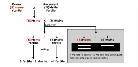
Use of Markers
An example of the use of markers for foreground selection is described in Fig. 5. Without a marker, it would be difficult to distinguish heterozygous carriers of the recessive male sterility allele ms (Msms) from homozygous (MsMs) genotypes, because both genotypes result in fertile plants. By using a co-dominant marker linked to Ms/ms, heterozygotes can be readily identified, and there is no need to spend time and resources on selfing and scoring offspring in the next generation based on pollen production.
Foreground Selection For Transgenic Traits
| Trait | Crop species | Transgene |
|---|---|---|
| Insect/pest resistance | Cotton, maize | Resistance to the European corn borer, through the expression of a transgene encoding the Cry1Ab insect toxin from Bacillus thuringiensis. |
| Disease resistance | Papaya, tobacco | Resistance to viral diseases by expression by viral coat protein genes. |
| Herbicide tolerance | Cotton, maize, soybeans | Glyphosate herbicide (Roundup) tolerance conferred by expression of a glyphosate-tolerant form of the plant EPSP synthase encoded by a transgene from the soil bacterium Agrobacterium tumefaciens stain CP4. |
| Tolerance to environmental stress | Maize | Expression of a drought-resistance gene from Bacillus subtilis. |
| Improved nutritional value | Canola | High laureate levels achieved by a gene encoding ACP thioesterase from the California bay tree Umbellularia californica. |
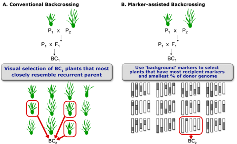
Background Selection
After carriers of the target trait were identified by foreground selection, the next issue is to efficiently recover the recurrent parent genome in as few generations as possible. Phenotypic selection of plants that closely resemble the recurrent parent (Fig. 6A) is challenging for traits that are difficult to score, and mostly due to the impact of linkage drag (see below). Consequently, for the transfer of a single dominant gene using the classical BC method, five or more BC generations are needed to recover 99% of the recurrent parent genome. To speed up the recovery of the recurrent parent genome, markers are used for selecting individuals that closely resemble the genetic background of the recurrent parent. The application of markers to analyze the genetic background of the recurrent parent in BC generations is referred to as marker-assisted background selection (Fig. 6B).
Objective of Background Selection
The objective of background selection is to accelerate the return to recipient parent genome outside the target gene so as to:
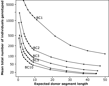
- Reduce the length of the donor chromosomal portion dragged along with the target gene on the carrier chromosome. This can be achieved by selecting recombinants between target gene and one or both flanking markers. The probability of finding a recombinant depends on the distances between the target gene and those flanking markers, number of BC generations, and number of individuals evaluated.
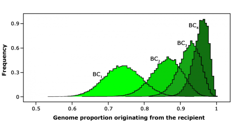
- The aim of background selection is to reduce the donor genome contribution in subsequent BC generations efficiently by selecting in each generation BC individuals with the lowest donor genome percentage across the genome (Fig. 7).
Versatility of MABC
Selecting in BC1 individuals with the highest recurrent parent genome content would help approach or even exceed the expected genome fraction of BC2 (Fig. 8). Therefore, using markers is a “shortcut” to “jump” BC generations and in this way speed up the BC process.
Example of Background Selection
The following is a summary of use of background selection in a BC program for disease resistance in wheat showing the introduction of strip rust resistance by backcross breeding in wheat.
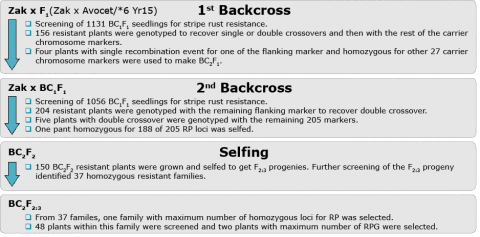
Controlling Linkage Drag
For this section it is recommended that you review the module on Linkage from Crop Genetics: genes located on the same chromosome are genetically linked. Closely linked genes are not segregating independently, like genes located on different chromosomes. This has different implications, e.g., in relation to trait correlations.
Conventional BC programs are designed with an assumption that the proportion of the recurrent parent genome will be recovered at a rate of 1 – (1/2)t+1 for each t generation of backcrossing. Therefore, after 5 generations of backcrossing, the rate of recovery of the recurrent parent genome would be 0.98%. However, the reality is that the actual outcome deviates from the expected recovery rate due to chance and in particular, linkage between the target gene from the donor parent with other regions of the donor chromosome (linkage drag). The remaining regions of the donor chromosome may contain genes that negatively affect agronomic performance (Fig. 10) and impose a drag on the improvement process.
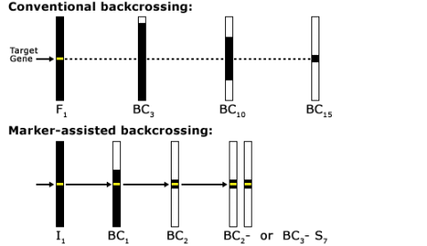
Reducing BC Generations
As indicated in Fig. 11, a classical BC program consists of at least five generations with random selection between all carriers of the target genes. The use of markers in backcrossing helps to detect and greatly minimize the number of donor chromosomes in the recurrent parent (Fig. 12). For this reason, markers can be applied to identify rare individuals resulting from recombination close to the desired gene, helping to minimize linkage drag. Consequently, MABC reduces the number of BC generations required for gene introgression from six to three.
Reducing Linkage Drag
Reduction of linkage drag requires both background and foreground selection. The minimum number of markers required for linkage drag reduction is three: one for the target gene to make sure it is still present in recombinants, and two flanking markers to search for recombinants. To minimize this risk of losing the target allele through crossover events, flanking markers on both sides can be applied (Fig. 13), but ultimately phenotyping is required to make sure that the target gene is still present. If the target gene sequence is known (for example, a transgene), phenotypic validation may not be required. But to ensure the gene is correctly expressed, phenotypic validation would still be done before a variety is released.
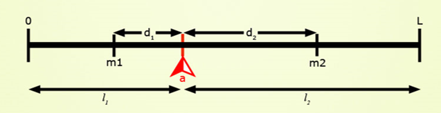
Target Locus
Positions on the chromosome shown in these are in a scale of 0 to L in Morgan units. Presence of locus a is diagnosed by the presence of closely linked (d1, d2 < 3 cM) marker alleles m1 and m2 with the assumptions that, (a) the average number of crossovers = the length of the chromosome in Morgan units, and (b) the locations of crossovers are independently distributed on the chromatid. Assumptions (a) and (b) are based on Haldane’s mapping function (Haldane, 1919), and imply that there is no crossover interference.
Plants would be heterozygous at target locus (a) and otherwise be:
- Type 1: homozygous carrier of recipient allele at both flanking markers.
- Type 2: homozygous carrier of recipient allele at one flanking marker, and heterozygous at the other.
- Type 3: homozygous carrier of recipient allele at one flanking marker, and homozygous or heterozygous at the other.
- Type 4: heterozygous for the donor allele at the target locus and heterozygous for the recurrent parent at both flanking markers.
- Type 5: homozygous for the recurrent parent allele at the target locus; i.e., not a carrier of the target allele.
Minimum Population Size
As described previously, the minimum population size required to generate with probability q = 0.99 at least one BC1 individual of Type 2 can be estimated by the following formula:
[latex]q = (_{m}^{n})p_i^m (1-p_i)^{n-m}[/latex]
where:
m = number of individuals with target genotype
n = minimum sample size
q = probability to find at least one individual of a genotype
pi = probability for occurrence of a particular genotype i  {1, 2L, 2R, 3L, 3R, 4}, L and R denote chromosome positions, left or right of the target locus (Frisch et al. 1999a), is defined as “is a subset of”. Therefore, i is a subset of {1, 2L, 2R, 3L, 3R, 4}.
Solving for n yields the minimum population size required to find with probability q at least one individual occurring with probability pi (see Table 4).
[latex]n \geq \dfrac{\ln(1-q)}{\ln(1-p_i)}[/latex]
| Event G (type) | Event G (Genotype) | Event G (No crossover in) | Condition H: NRP is of Genotype | Conditional probability P(G|H) |
|---|---|---|---|---|
| 1 | y1– x + yr– | —– | y1+ x + yr+ | P1 = PBPC /2 |
| 2L | y1– x + yr– | —– | y1+ x + yr+ | P2L = PB(1 – pc) /2 |
| 2R | y1– x + yr– | —– | y1+ x + yr+ | P2R = (1 – pB) pc /2 |
| 2 | 2L or 2R | p2 = p2L + p2R |
Target Genotype
In Table 5, numerical values for the minimum number of individuals required to find a target genotype are provided, (a) in case of looking for a double cross-over event (Type 1), or two subsequent generations of recombination (Type 2, Type 3L combined). For example, if the distance of both flanking markers is 5 cM, then at least 4066 individuals are required to find a double recombinant with q = 0.99. If two subsequent generations are considered, then the respective minimum number of individuals required is 292, i.e., 100 (Type 2) + 192 (Type 3L) = 292. Thus, the number of plants to be genotyped in this second scenario is substantially reduced.
Table 5 Minimum number of individuals (n) required to obtain with probability q = 0.99 at least one plant of Type 1, 2 or 3L. Data from Frisch et al., 1999a.
| Distance of flanking marker d1 [cM] | 5 | 10 | 15 | 20 | 25 |
|---|---|---|---|---|---|
| Distance of flanking marker d2 [cM] | 5 | 10 | 15 | 20 | 25 |
| Minimum number of Type 1 individuals | 4066 | 1119 | 547 | 337 | 236 |
| Minimum number of Type 2 individuals | 100 | 54 | 39 | 32 | 27 |
| Minimum number of Type 3L individuals | 192 | 100 | 69 | 54 | 45 |
MABC for Single Gene
Comparing Different BC Strategies
Frisch et al. (1999b) conducted simulations to compare several different BC strategies in terms of the speed of recovery of a large proportion of the recurrent parent genome (Table 6). The simulations were based on a maize genetic map (n = 10 chromosomes) with markers spaced about 20 cM.
| Selection for | Number of selection steps | ||
| Two | Three | Four | |
| Presence of the target gene | 1 | 1 | 1 |
| Homozygosity for the recurrent parent allele at flanking markers | No data | 2 | 2 |
| Homozygosity for the recurrent parent allele at all markers on the carrier chromosome | No data | No data | 3 |
| Homozygosity for the recurrent parent allele at markers across the genome | 2 | 3 | 4 |
Note that, each stage is run in each BC generation. That means, in two-stage selection, there is both foreground and background selection done in BC1, then also in BC2. The same holds true for three-, and four-stage selection. In performing the simulations, Frisch et al. (1999b) used the following parameters:
a. Marker data points (MDP) The mean number of MDP required over 10,000 repetitions of the simulation was calculated. Each analysis of a marker locus in a backcross individual was counted as 1 MDP. If one BC individual was genotyped with 100 markers, this would be counted as 100 MDP. Similarly, if 100 BC individuals are genotyped with 100 markers each, this results in 10,000 MDP.
Recurrent Parent Genome
b. Recurrent parent genome (RPG) The 10% percentile (Q10) of the empirical distribution of the RPG in the 10,000 repetitions was calculated. For example, Q10 = 98.0% means that a RPG proportion of greater than 98% is attained with a probability of 90%. Table 7 contains simulations results of the distribution of the recurrent parent genome in BC generations 1-10 when foreground selection was implemented or not implemented.
Table 7 Simulation results for the mean and 10% percentile (Q10) of the distribution of the recurrent parent genome in several BC generations with random selection of individuals carrying the target allele and expected values for the mean without selection. Data from Frisch et al., 1999b.
| No selection | Selection | Selection | |
|---|---|---|---|
| Generation | Mean (%) | Mean (%) | Mean Q10 (%) |
| BC1 | 75.0 | 74.0 | 67.4 |
| BC2 | 87.5 | 86.1 | 80.7 |
| BC3 | 93.8 | 92.4 | 88.3 |
| BC4 | 96.9 | 95.6 | 92.7 |
| BC5 | 98.4 | 97.3 | 95.2 |
| BC6 | 99.2 | 98.2 | 96.7 |
| BC7 | 99.6 | 98.7 | 97.6 |
| BC8 | 99.8 | 99.0 | 98.1 |
| BC9 | 99.9 | 99.1 | 98.5 |
| BC10 | 100.0 | 99.3 | 98.7 |
Detect the Level of RPG
Following the criteria mentioned above, the number of individuals and MDP required to detect the level of RPG in various BC generations can be estimated. Let us compare two-stage and three-stage selection strategies with respect of RPG and MDP criteria and a Q10 threshold of 96.7% as proposed by Frisch et al. (1999b).
Tables 8 and 9 contain results from the simulation at the two-stage selection with constant and varied population sizes, respectively. Table 10 contains results for the three-stage selection with constant population size.
Table 8 Two-stage selection, constant population size. Data from Frisch et al., 1999b.
| Number of individuals per BC generation | ||||||||
|---|---|---|---|---|---|---|---|---|
| 20 | 40 | 60 | 80 | 100 | 125 | 150 | 200 | |
| Q10 of the RPD (10%) |
||||||||
| BC1 | 76.7 | 78.7 | 79.7 | 80.3 | 80.7 | 81.3 | 81.7 | 82.2 |
| BC2 | 90.3 | 91.9 | 92.8 | 93.3 | 93.6 | 93.9 | 94.0 | 94.6 |
| BC3 | 95.8 | 06.2 | 97.1 | 97.3 | 97.4 | 97.5 | 97.6 | 97.8 |
| Number of MDP required in total |
||||||||
| BC1 | 795 | 1560 | 2400 | 3200 | 4000 | 5000 | 5990 | 8000 |
| BC2 | 1010 | 2130 | 3150 | 4170 | 5180 | 6430 | 7670 | 10100 |
| BC3 | 1180 | 2280 | 3340 | 4390 | 5430 | 6720 | 7990 | 10500 |
Results Using Different Ratios
Considering results in Table 8, based on 3340 MDP, Q10 amounted to 97.1% in BC3 with population (n1) of 60 individuals. Also, increasing the population (n) size beyond 100 has little effect on the RPG, but requires a large number of MDP. Importantly, the total number of MDP required is approximately proportional to the number of individuals.
Results in Table 9 suggest that the different ratios do not have a large impact on the Q10 values in BC3. In contrast, the MDP required is strongly reduced for larger populations in BC3. Also, with the ratio of 1:3:9 about 50% less MDP are required as compared to the ration of 1:1:1.
Table 9 Two-stage selection, increasing or decreasing population size. Data from Frisch et al., 1999b.
| Ratio n1 : n2 : n3 | |||||||
|---|---|---|---|---|---|---|---|
| 3:2:1 | 1:1:1 | 2:3:4 | 1:2:3 | 1:3:5 | 1:2:4 | 1:3:9 | |
| Number of individuals nt | |||||||
| BC1 | 150 | 100 | 66 | 50 | 33 | 43 | 23 |
| BC2 | 100 | 100 | 100 | 100 | 100 | 86 | 68 |
| BC3 | 50 | 100 | 133 | 150 | 166 | 171 | 209 |
| Q10 of the RPG (%) | |||||||
| BC1 | 81.6 | 80.7 | 80.0 | 79.3 | 78.3 | 78.9 | 77.1 |
| BC2 | 93.8 | 93.6 | 93.2 | 93.1 | 92.8 | 92.8 | 91.9 |
| BC3 | 97.3 | 97.4 | 97.4 | 97.4 | 97.4 | 97.4 | 97.3 |
| Number of MDP required in total | |||||||
| BC1 | 6010 | 4000 | 2680 | 2000 | 1370 | 1720 | 920 |
| BC2 | 7120 | 5180 | 3910 | 3290 | 2720 | 2850 | 1900 |
| BC3 | 7240 | 5430 | 4280 | 3720 | 3230 | 3380 | 2650 |
Three-Stage Selection
Table 10 Three-stage selection with constant population size. Data from Frisch et al., 1999b.
| Number of individuals per BC generation | ||||||||
|---|---|---|---|---|---|---|---|---|
| 20 | 40 | 60 | 80 | 10 | 125 | 150 | 200 | |
| Q10 of the RPG (%) | ||||||||
| BC1 | 71.2 | 72.7 | 73.4 | 73.6 | 73.3 | 73.2 | 72.8 | 72.2 |
| BC2 | 86.1 | 87.2 | 88.5 | 89.3 | 90.2 | 90.7 | 91.3 | 91.8 |
| BC3 | 94.4 | 95.7 | 96.5 | 96.9 | 97.2 | 97.3 | 97.5 | 97.6 |
| Number of MDP required in total | ||||||||
| BC1 | 250 | 320 | 420 | 510 | 590 | 690 | 750 | 840 |
| BC2 | 440 | 610 | 830 | 1100 | 1390 | 1780 | 2210 | 3110 |
| BC3 | 550 | 820 | 1130 | 1470 | 1810 | 2260 | 2740 | 3740 |
Results in Table 10 indicate that the Q10 values for BC1 and BC2 are lower than those obtained in two-stage selection. However, the difference is marginal for the two approaches at BC3. Using 1470 MDP, the threshold of 97.0% was reached when 80 individuals were considered in the three-stage selection. This means that a reduction of about 50% in the required number of MDP can be achieved using the three-stage selection as compared to two-stage selection.
Tables 11 and 12 contain summaries of number of individuals and MDP for different selection strategies at different BC generations.
Attaining a Desired Q10 Percentile
Table 11 Number of individuals required to attain a desired Q10 percentile of the RPG. Data from Frisch et al., 1999b.
| Number of individuals n1 per backcross generation | ||||||
|---|---|---|---|---|---|---|
| Generation | 20 | 4 | 6 | 80 | 100 | 125 |
| Two-stage selection | Q10 of the RPG (%) | |||||
| BC1 | 76.7 | 78.7 | 79.7 | 80.3 | 80.7 | 81.3 |
| BC2 | 90.3 | 91.9 | 92.8 | 93.3 | 93.6 | 93.9 |
| BC3 | 95.8 | 96.2 | 97.1 | 97.3 | 97.4 | 97.5 |
| BC4 | 97.8 | 97.9 | 98.4 | 98.5 | 98.5 | 98.6 |
| BC5 | 98.7 | 98.9 | 99.0 | 99.0 | 99.0 | 99.0 |
| Three-stage selection | Q10 of the RPG (%) | |||||
| BC1 | 71.2 | 72.7 | 73.4 | 73.6 | 73.3 | 73.2 |
| BC2 | 86.1 | 87.2 | 88.5 | 89.3 | 90.2 | 90.7 |
| BC3 | 94.4 | 95.7 | 96.5 | 96.9 | 97.2 | 97.3 |
| BC4 | 97.7 | 98.2 | 98.4 | 98.4 | 98.4 | 98.5 |
| BC5 | 98.7 | 98.8 | 98.9 | 98.9 | 98.9 | 98.9 |
| Four-stage selection | Q10 of the RPG (%) | |||||
| BC1 | 71.0 | 71.9 | 72.1 | 71.7 | 71.6 | 71.5 |
| BC2 | 85.5 | 86.2 | 87.2 | 87.6 | 88.2 | 88.7 |
| BC3 | 93.7 | 95.0 | 96.0 | 96.5 | 96.8 | 97.0 |
| BC4 | 97.6 | 98.2 | 98.3 | 98.4 | 98.4 | 98.4 |
| BC5 | 98.7 | 98.8 | 98.9 | 98.9 | 98.9 | 98.9 |
Detecting a Desired RPG Level
Table 12 Number of MDP required to detect a desired level of RPG. Data from Frisch et al., 1999b.
| Number of individuals n1 per backcross generation | ||||||
|---|---|---|---|---|---|---|
| Generation | 20 | 40 | 60 | 80 | 100 | 125 |
| Two-stage selection | Number of MDP required in total | |||||
| BC1 | 800 | 1560 | 2400 | 3200 | 4000 | 5000 |
| BC2 | 1010 | 2130 | 3150 | 4170 | 5180 | 6430 |
| BC3 | 1180 | 2280 | 3340 | 4390 | 5430 | 6750 |
| BC4 | 1210 | 2310 | 3380 | 4430 | 5470 | 6750 |
| BC5 | 1220 | 2320 | 3380 | 4430 | 5470 | 6760 |
| Three-stage selection | Number of MDP required in total | |||||
| BC1 | 250 | 320 | 420 | 510 | 590 | 690 |
| BC2 | 440 | 610 | 830 | 1100 | 1390 | 1780 |
| BC3 | 550 | 820 | 1130 | 1470 | 1810 | 2260 |
| BC4 | 590 | 860 | 1170 | 1500 | 1840 | 2280 |
| BC5 | 590 | 860 | 1170 | 1500 | 1840 | 2280 |
| Four-stage selection | Number of MDP required in total | |||||
| BC1 | 230 | 270 | 340 | 390 | 430 | 470 |
| BC2 | 370 | 460 | 590 | 750 | 910 | 1140 |
| BC3 | 460 | 660 | 900 | 1140 | 1290 | 1710 |
| BC4 | 500 | 710 | 950 | 1190 | 1430 | 1740 |
| BC5 | 510 | 710 | 950 | 1190 | 1430 | 1740 |
Altering Size of Populations
Table 13 The impact of altering size of populations on MDP and detection of desired QP10 percentile of RPG. Data from Frisch et al., 1999b.
| Ratio n1 : n2 : n3 | |||||||
|---|---|---|---|---|---|---|---|
| 3:2:1 | 1:1:1 | 2:3:4 | 1:2:3 | 1:3:5 | 1:2:4 | 1:3:9 | |
| Generation | Number of individuals nt | ||||||
| BC1 | 150 | 100 | 66 | 50 | 33 | 43 | 23 |
| BC2 | 100 | 100 | 100 | 100 | 100 | 86 | 68 |
| BC3 | 50 | 100 | 133 | 150 | 166 | 171 | 209 |
| Two-stage selection | Q10 of the RPG (%) | ||||||
| BC1 | 81.6 | 80.7 | 80.0 | 79.3 | 78.3 | 78.9 | 77.1 |
| BC2 | 93.8 | 93.6 | 93.2 | 93.1 | 92.8 | 92.8 | 91.9 |
| BC3 | 97.3 | 97.4 | 97.4 | 97.4 | 97.4 | 97.4 | 97.3 |
| Three-stage selection | Q10 of the RPG (%) | ||||||
| BC1 | 72.8 | 73.1 | 73.7 | 73.1 | 72.3 | 72.8 | 71.4 |
| BC2 | 90.5 | 90.0 | 89.5 | 88.8 | 88.1 | 88.3 | 86.9 |
| BC3 | 97.0 | 97.1 | 97.1 | 97.0 | 96.9 | 97.0 | 96.7 |
| Four-stage selection | Q10 of the RPG (%) | ||||||
| BC1 | 71.2 | 71.6 | 72.0 | 72.0 | 71.5 | 71.9 | 71.1 |
| BC2 | 88.5 | 88.2 | 88.0 | 87.4 | 87.0 | 87.0 | 86.9 |
| BC3 | 96.5 | 96.7 | 96.8 | 96.8 | 96.6 | 96.6 | 96.3 |
| Two-stage selection | Number of MDP required in total | ||||||
| BC1 | 6010 | 4000 | 2680 | 2000 | 1370 | 1720 | 920 |
| BC2 | 7120 | 5180 | 3910 | 3290 | 2720 | 2850 | 1900 |
| BC3 | 7240 | 5430 | 4280 | 3720 | 3230 | 3380 | 2650 |
| Three-stage selection | Number of MDP required in total | ||||||
| BC1 | 750 | 590 | 450 | 370 | 290 | 240 | 250 |
| BC2 | 1740 | 1390 | 170 | 930 | 740 | 790 | 580 |
| BC3 | 1930 | 1820 | 1690 | 1660 | 1620 | 1680 | 1760 |
| Four-stage selection | Number of MDP required in total | ||||||
| BC1 | 480 | 430 | 350 | 300 | 260 | 290 | 240 |
| BC2 | 1070 | 910 | 740 | 640 | 540 | 570 | 440 |
| BC3 | 1310 | 1290 | 1400 | 1400 | 1400 | 1450 | 1500 |
Key Points from the Simulation Work of Frisch et al. (1999b):
- Increasing the number of individuals genotyped each generation had minor effect.
- Using markers, about 97% of the recurrent parent genome can be accomplished in three BC generations.
- The three- and four-stage selection strategies are more efficient.
- In a three-stage selection program, increasing population sizes with each generation is most efficient.
- Fewer marker data points are required for three- and four-stage programs than for two-stage selection to recover nearly the same content of the recurrent parent genome.
Although the simulation study by Frisch et al. (1999b) revealed that the four-stage selection strategy is the most efficient procedure in MABC, the success of MABC also relies on several factors, including distance between markers and the target gene, the number of target genes to be backcrossed, the number of individuals that can be evaluated and the genetic background of the recurrent parent, types of molecular markers and instrumentation for marker analysis.
A Two-Generation Breeding Plan
A two-generation breeding plan for introgression of a dominant gene:
- Choosing the desired probability of success q(2), set q(1) = q(2)
- Carrying out BC1 with n(1) such that at least one individual of Type 2L or 2R is generated with the probability q(1)
- Selecting a BC1 individual according to (d1 < d2), recall this is the distance of the flanking markers from the target genes (Fig. 14). Such that, Type 1 > Type 2L > Type 2R > Type 4
- Carrying out generation BC2 n(2) such that at least one individual of Type 2R is generated with probability q(2)
- Optimizing of the breeding plan such that: [latex]n_1 + E(n_2) \rightarrow \textrm{min,} \ q^{(2)} = 0.99[/latex]
Developing Improved Lines
Developing improved lines and varieties is often done by combining desirable traits from multiple parental lines by the process referred to as gene stacking or gene pyramiding. Thus, gene stacking is the production of a plant with a desired combination of two or more unique genes. This can be done when the genes are initially transferred into the plant cells by transformation or during breeding by crossing two lines that each contains a different gene resulting in progeny with both genes. Gene stacking has several applications, for example, introduction of durable resistance that is harder to overcome by the pathogen than a monogenic resistance. Guidelines for Simultaneous Introgression of Two GenesFrisch and Melchinger (2001) compared various selection strategies and breeding plans (Fig. 14) for the simultaneous introgression of two genes with respect to the recurrent parent genome (RPG) recovery and the number of marker data points (MDP) required.
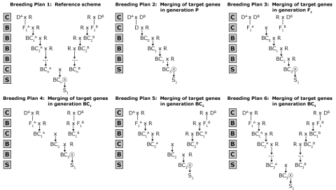
Proposed Guidelines
The following guidelines were proposed:
- In comparison to two-stage and three-stage selection, fewer marker data points (MDP) are required. Also greater values for recurrent parent genome (RPG) are achieved.
- The selection intensity depends on the breeding plan. For example, A: 50%, B: 25% of one generation will be genotyped.
- Merging the target genes in later generations will require more MDP and will result on greater RPG value.
Based on the strategies described in Fig. 14, probability of occurrence can be determined (see Table 2 in Frisch and Melchinger, 2001).
MABC for several genes
Table 14 Simulation results for the 10% percentile (Q10) of the distribution of the recurrent parent genome in the selected BCyS1 individual and total number of marker data points (MDP) required in a backcross program to introgress two unlinked target genes. Values of MDP are rounded to multiples of ten. Data from Frisch et al., 1999b.
| Population size in generation | Selection strategy | |||||
|---|---|---|---|---|---|---|
| Merging of target genes in generation | BC1 | BC2 | BC3 | Two-stage selection | Three-stage selection | Four-stage selection |
| Q10 (%) /mdp | ||||||
| P | 60 | 120 | 180 | 94.9/2560 | 94.2/780 | 93.9/750 |
| P | 120 | 120 | 120 | 94.9/350 | 94.3/820 | 93.9/800 |
| P | 180 | 120 | 60 | 94.7/4540 | 94.2/810 | 93.8/820 |
| Q10 (%) /mdp | ||||||
| F1 | 60 | 120 | 180 | 95.2/4200 | 95.0/1200 | 94.7/1090 |
| F1 | 120 | 120 | 120 | 95.1/4780 | 95.1/120 | 94.7/1140 |
| F1 | 180 | 120 | 60 | 94.9/5390 | 94.9/1200 | 94.5/1140 |
| Q10 (%) /mdp | ||||||
| BC1 | 2 x 30 | 120 | 180 | 05.4/4590 | 95.5/1590 | 95.4/1380 |
| BC1 | 2 x 60 | 120 | 120 | 95.5/6730 | 95.8/1780 | 95.5/1480 |
| BC1 | 2 x 90 | 120 | 60 | 95.4/8970 | 95.6/210 | 95.4/1550 |
| Q10 (%) /mdp | ||||||
| BC2 | 2 x 30 | 2 x 60 | 180 | 95.8/4670 | 96.0/1910 | 95.8/1530 |
| BC2 | 2 x 60 | 2 x 60 | 120 | 95.9/6810 | 96.1/2240 | 95.9/1690 |
| BC2 | 2 x 90 | 2 x 60 | 60 | 95.8/9050 | 96.2/2590 | 95.9/1860 |
| Q10 (%) /mdp | ||||||
| BC3 | 2 x 30 | 2 x 60 | 2 x 90 | 96.2/4780 | 96.3/2280 | 96.2/1960 |
| BC3 | 2 x 60 | 2 x 60 | 2 x 60 | 96.2/6770 | 96.4/2340 | 96.3/1910 |
| BC3 | 2 x 90 | 2 x 60 | 2 x 30 | 96.1/8900 | 96.3/2470 | 96.2/1870 |
| Reduced selection strategies | Q10 (%) /mdp | |||||
| BC1 | 2 x 30 | 120 | 180 | 95.4/4380 | 95.5/1550 | 95.3/1380 |
| BC1 | 2 x 60 | 120 | 120 | 95.4/6280 | 95.7/1720 | 95.4/1480 |
| BC1 | 2 x 90 | 120 | 60 | 95.3/8270 | 95.6/1920 | 95.4/1550 |
| Reduced selection strategies | Q10 (%) /mdp | |||||
| BC2 | 2 x 30 | 2 x 60 | 180 | 95.8/4290 | 96.0/1780 | 95.8/1490 |
| BC2 | 2 x 60 | 2 x 60 | 120 | 95.8/190 | 96.1/2080 | 95.9/1650 |
| BC2 | 2 x 90 | 2 x 60 | 60 | 95.7/8190 | 96.1/2370 | 95.9/1780 |
| Reduced selection strategies | Q10 (%) /mdp | |||||
| BC3 | 2 x 30 | 2 x 60 | 2 x 90 | 96.2/4310 | 96.3/1780 | 96.2/1850 |
| BC3 | 2 x 60 | 2 x 60 | 2 x 60 | 96.2/6100 | 96.3/2140 | 96.3/1820 |
| BC3 | 2 x 90 | 2 x 60 | 2 x 30 | 96.1/8030 | 96.3/2280 | 96.2/1790 |
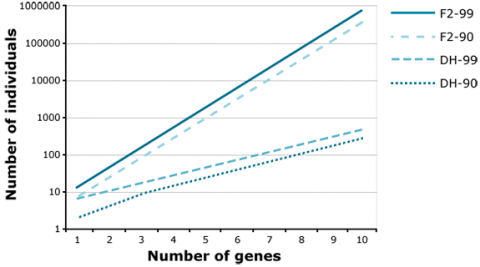
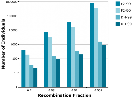
Detecting a Desired Genotype
Application of the doubled haploid (DH) method allows the development of completely homozygous plants from which breeding lines or cultivars are derived within two years. The main advantage of using DHs versus BCnF2-derived lines is, that in case of introgression of an increasing number of unlinked genes, the number of offspring required to find a line with all target genes fixed is increasingly demanding for F2-derived lines versus DHs. For example, to find at least one homozygous offspring (q = 0.95) with 8 fixed genes, about 1000 DHs are required. For the same objective, about 100,000 F2-derived are required (Fig. 15). Similarly, much fewer DHs are required compared to F2 to identify recombinants between two genes linked in repulsion (Fig. 16).
Identification of Genotypes
References
Collard, B.C.Y., and D.J. Mackill. 2008. Marker-assisted selection: an approach for precision plant breeding in the twenty-first century. Phil. Trans. R. Soc. B. 363: 557-572. http://www.ncbi.nlm.nih.gov/pmc/articles/PMC2610170/pdf/rstb20072170.pdf
Frisch, M., M. Bohn, and A.E. Melchinger. 1999a. Minimum sample size and optimal positioning of flanking markers in marker-assisted backcrossing for transfer of a target gene. Crop Sci. 39:967-975.
Frisch, M., M. Bohn, and A.E. Melchinger. 1999b. Comparison of selection strategies for marker-assisted backcrossing of a gene. Crop Sci. 39:1295-1301.
Frisch, M., and A.E. Melchinger. 2001a. Marker-assisted backcrossing for simultaneous introgression of two genes. Crop Sci. 41: 1716-1725.
Frisch, M., and A. E. Melchinger. 2001b. The length of the intact donor chromosome segment around a target gene in marker-assisted backcrossing. Genetics 157: 1343-1356.
Haldane, J.B.S. 1919. The combination of linkage values and the calculation of distances between linked factors. J. Genet. 8: 299-309.
Hospital, F., and A. Charcosset. 1997. Marker-assisted introgression of quantitative trait loci. Genetics 147: 1469-1485.
Hospital, F. 2001. Size of donor chromosome segments around introgressed loci and reduction of linkage drag in marker-assisted backcross programs. Genetics 158: 1363-1379.
Hospital, F. 2005. Selection in backcross programmes. Phil. Trans. R. Soc. B. 360: 1503-1511.
Lübberstedt, T., and U.K. Frei. 2012. Application of doubled haploids for target gene fixation in backcross programmes of maize. Plant Breed. 131: 449-452.
Morris, M., K. Dreher., J-M. Ribaut, and M. Khairallah. 2003. Money matters (II): costs of maize inbred line conversion schemes at CIMMYT using conventional and marker-assisted selection. Mol. Breed. 11: 235-247.
Randhawa, H. S., J.S. Mutti, K. Kidwell, C.F. Morris, X. Chen, and K.S. Gill. 2009. Rapid and Targeted Introgression of Genes into Popular Wheat Cultivars Using Marker-Assisted Background Selection. PLoS ONE 4(6): e5752. doi:10.1371/journal.phone.0005752 E
Ribaut, J.M., and D. Hoisington. 1998. Marker-assisted selection: new tools and strategies. Trends Plant Sci. 3: 236-239.
Segman, K., A. Bjønstad, and M.N. Ndjiondjop. 2006. Progress and prospects of marker assisted backcrossing as a tool in crop breeding programs. African J. Biotechnol. 5: 2588-2603.
Zheng, N., S. Moeinizade, A. Kusmec, G. Hu, L. Wang, and P. S. Schnable. 2023. New insights into trait introgression with the look-ahead intercrossing strategy, G3 Genes|Genomes|Genetics: jkad042. https://doi.org/10.1093/g3journal/jkad042.
