Chapter 7: Marker Assisted Selection and Genomic Selection

Limitations in QTL Mapping

QTL Dependencies

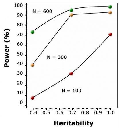
As discussed in the module on Cluster Analysis, Association & QTL Mapping, the goal of QTL mapping is to identify one or more genomic region(s) called quantitative trait locus (QTL) controlling a particular trait. However, the statistical power for detecting QTL depends on population size, leading to overestimation of QTL effects in small populations (Beavis, 1994), the Beavis effect. For this reason, QTL studies depend on very large sample sizes, and are only capable of detecting differences that are captured between the parents used to form a mapping population. Thus, within a given population, if the same parents were used to map QTL and to establish a breeding population, all QTL are of interest. Some QTL might not be relevant when they are transferred to other populations (if there is no segregation for that QTL). Another issue is, QTL determined at per se level might not be relevant for the testcross level in hybrid species like maize. Therefore, the way phenotyping is done affects the detection and consistency of QTL.

For all strategies presented in this lesson, it is crucial to understand that the reason for limited success of MAS (compared to GS) is their dependence on QTL mapping. QTL mapping has been shown to only find a fraction of QTL affecting a quantitative trait, and to overestimate genetic effects for detected QTL. Thus, during MAS, relevant regions in the genome are missed, whereas other regions likely get too much weight, so that expected findings likely differ from actual ones, leading to limited gain in selection.

Impact Graph

MAS Strategies

MAS Strategies – F₂ Enrichment

A. F₂ Enrichment

The objective of the F₂ enrichment strategy is to develop superior Recombinant Inbred Lines (RILs). MAS is particularly useful for F₂ individuals or F₂-derived lines, or other early generations (DHs, BC1-derived populations), because LD between marker loci and the trait of interest are at a maximum in a segregating population. A good example of the application of F₂-enrichment comes from a wheat breeding program at CSIRO Plant Industry in Canberra, Australia (Bonnett et al., 2004). 

The F₂ enrichment procedure involves:

1. QTL identification
2. Culling of undesirable genotypes to increase frequency of desirable alleles/genotypes
3. Identification of RILs with all favorable QTL alleles fixed

[latex]y = \mu _{\mathit{0}} + \sum_{\mathit{i=1}}^{N}a_{i}x_{i}+\varepsilon[/latex]

where:

y = the expected phenotypic value of an individual
μ₀ = the model mean
a_i = additive effect of the marker.
ε = random environmental factor
x_i= indicator variable (with values 1,0 and -1 for marker genotypes MM, mm, and mm)
N  = the number of markers

Obtaining Marker Scores

B. Use of Marker Scores in Selection

Theoretically, selection of individuals is most efficient when based on additive gene effects. QTL analysis identifies chromosome segments affecting traits of interest, and enables us to estimate gene effects (additive, dominance, and epistasis) for each QTL. If summarized across all detected QTL, the expected performance of an individual can be predicted based on the QTL information. QTL analysis depends on the precise mapping of each QTL along with marker-trait regression analysis to estimate the genetic effects of QTL. Marker-trait regression uses the following equation:

[latex]y = \mu _{\mathit{0}} + \sum_{\mathit{i=1}}^{N}a_{i}x_{i}+\varepsilon[/latex]

where:

y = the expected phenotypic value of an individual
μ₀ = the model mean
a_i = additive effect of the marker.
ε = random environmental factor
x_i = indicator variable (with values 1,0 and -1 for marker genotypes MM, mm, and mm)
N  = the number of markers

Thus, markers (representing QTL) with significant effects on the trait of interest can be used to obtain marker scores (also referred to as molecular score) for each individual. The following expression is used to estimate marker scores (MS):

[latex]MS = \sum_{\mathit{\mathit{i=1}}}^{N}a_{i}x_{i}[/latex]

where:

n  = the number of markers selected
a_i = additive effect of the marker i
x_i = indicator variable with values 1, 0 and -1 for marker genotypes MM, Mm and mm)

Derivation of a Selection Index

C. Derivation of a Selection Index for MAS

Lande and Thompson (1990) demonstrated that MAS is most effective when breeding values are predicted by an index of QTL genotypic values and phenotypic values. Index weights are estimated that maximize the correlation between the index and a candidate’s breeding value (A_total). A_total is the sum of individual’s breeding value for the marked QTL (A_QTL) and the breeding value for all other genes (A_rest), not explained by QTL. Thus, A_total = A_QTL + A_rest.

1. Estimating marker scores

A marker weight coefficient (b_MS) is estimated as follows:

[latex]b_{MS} = \frac{1-h_{2}}{1-\Theta h_{2}}[/latex]

 

where:

MS = marker score
h² = narrow sense heritability
θ = proportion of genetic variance explained by a marker score

2.  Estimating index weight of marker score relative to phenotype 

An individual’s phenotype (P) is weighed using the following formula (Bernardo, 2009):

[latex]b_{p} = \frac {h^2(1 - \Theta )}{1-\Theta h^{2}}[/latex]

 

Thus, MS is weighted more heavily than P.

If h² is 1, and θ ranges from 0.1 to 0.75, then the numerator of the marker weight coefficient b_MS will be close to 0, and thus, almost no weight will be assigned to markers. Thus, the higher the heritability of a trait, the lower the marker score. On the other hand, if h_² is low, and if θ is if high (>0.5), more weight will be assigned to markers.

3. Interpretation of the marker score

Assume a candidate’s breeding value (A_total) is the sum of its breeding value for the marked QTL (A_QTL) and its breeding value for all other genes (A_rest), not explained by QTL:

A_total = A_QTL + A_rest

Thus,

• The marker score gives an estimate of A_QTL
• Phenotype can be used to estimate an individual’s total breeding value, A_total

Therefore, possible selection strategies could be based on MS and phenotype as described by the following steps:

• Select on marker score alone: this ignores the information that is provided by phenotype on all the other genes that affect particular traits
• Independent culling level selection: that is, based on (a) selection on marker score, (b) selection on phenotype. Some individuals with desirable genes for non-marked QTL may be eliminated in (a)
• Index selection: develop index of marker score and phenotype (I = b_MS MS + b_p P). In general, expected response to selection index > independent culling > MS alone.

Marker-Assisted Recurrent Selection

D. Marker-Assisted Recurrent Selection

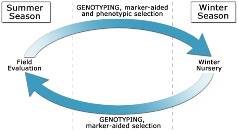
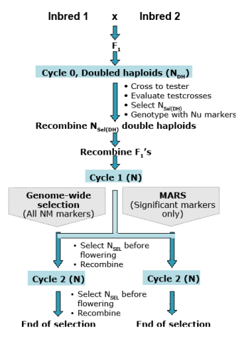
Marker-assisted recurrent selection (MARS) is used to enrich favorable alleles for QTL of interest over multiple generations. Indirect selection during winter generations can be combined with phenotypic selection or selection indices in rapid breeding cycles (Fig. 2).

MARS involves:

1. QTL identification, similar to F₂ enrichment.
2. Identification of best individuals based on marker score (Table 1) within population.
3. Recombination of best individuals followed by identification of best individuals as described in (2).
4. Click here to learn more about the application of MARS: Agronomy.org MARS information

MAS Strategies Comparison

Similarities and Differences of MAS Strategies

F2 enrichment	MARS
Involves QTL identification	Involves QTL identification
QTL are given equal weights	QTL are weighed according to the additive effect
Culling of undesirable genotypes	Identification of best individuals based on marker scores
Identification of RIL with favorable fixed alleles	Recombination of best individuals

Efficiency of MAS

Selection Index

To understand, what determines efficiency of MAS, we must understand how it is estimated. First, we estimate the accuracy of selection based on the selection index theory.

The selection index (I) is used to account for the relative superiority or inferiority of individuals for all the traits represented by the index.

[latex]I = b_1X_1 + b_2X_2 + … + b_nX_n = Σb_iX_i[/latex]

 

where:
b_i is the weight for trait i, and X_i is the phenotype value for trait i. The value of I is calculated for every individual or family in a population.

The selection index can also be denoted as I = b_MM + bpP.

[latex]b_P = \frac{V_A - V_M}{V_P - V_M}[/latex]

[latex]b_M = \frac{V_P - V_A}{V_P - V_M}[/latex]

where:
b_M and b_p are weights, M (or MS) is the marker score, and P is the phenotypic value.

The following equations can be used to estimate b_P and b_M:

[latex]b_P = \frac{V_A - V_M}{V_P - V_M}[/latex]

[latex]b_M = \frac{V_P - V_A}{V_P - V_M}[/latex]

where:
V_A = additive genetic variance
V_M = the additive variance explained by the marker
V_P = phenotypic variance

Estimating Relative Efficiency of MAS

Assuming that the selection intensity and generation interval are similar, the relative efficiency (RE) of MAS over phenotypic selection is obtained by comparing response from MAS to response from phenotypic selection (Bernardo, 2002).

1. RE of marker-based selection (RE_MBS:PS)

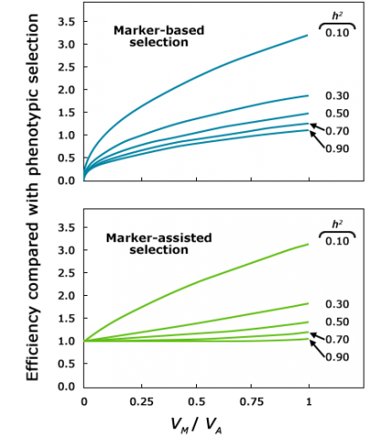
[latex]RE_{MBS:PS} = \frac{\sqrt{\frac{V_M}{V_A}}}{h}[/latex]

2. RE of marker-assisted selection (RE_MAS:PS)

[latex]RE_{MAS:PS} = \frac{\frac{V_M}{V_A}}{h^2} + \frac{{(1-(\frac{V_M}{V_A}))}^2}{1-h^2(\frac{V_M}{V_A})}[/latex]

Comparison to Phenotypic Selection

As Figure 3 and Table 1 show, MAS is more efficient than phenotypic selection for traits with low heritability, but MAS may not be economically justifiable for traits with higher heritability, and that are easier to score phenotypically. The reason is that when heritability (h) is high, gain from phenotypic selection nears the maximum possible given the genetic variance, leaving a small window for additional improvement by the use of markers.

Factors Affecting Efficiency

Table 1 Relative efficiency of marker-based selection compared with phenotypic selection in maize. Data from Bernardo, 2002.

Trait	VM/VA	h2	Relative Efficiency
Yield	0.51	0.63	1.09
Grain moisture	0.55	0.94	1.00
Stalk lodging	0.62	0.39	1.33
Root lodging	0.62	0.39	1.33
Plant height	0.58	0.89	1.01

Therefore, many factors affect the efficiency of MAS, including the size of the QTL mapping population, the phenotype to be scored, experimental design and analysis, the number of markers available, the degree of association between available markers and the QTL, the proportion of additive effect described by the marker, and the selection method. Also, the crop to be improved and the marker development pipeline have a bearing on the efficiency of MAS. While MAS may provide greater relative efficiency than phenotypic selection, MAS programs also require higher economic efficiency to justify their application in a breeding program. As seen in Table 2, MAS is less economical for traits such as seedling emergence. Such traits may be easier to score visually and would thus not justify the use of MAS for their evaluation. On the other hand, biochemical traits such as sucrose concentration justify the application of MAS because they are difficult to score.

Table 2 Estimates of the average evaluation costs (US $) for the selected traits using phenotypic selection (PS) and marker-assisted (MAS). Data from Yousef and Juvik, 2001.

C1 [latex]\ddagger[/latex]		C2 [latex]\S[/latex]		C3 [latex]\S[/latex]
Trait	PS	MAS	PS	MAS	PS	MAS
Emergence	56	103	42	78	37	70
Sucrose	178	164	134	109	119	90
Tenderness	158	154	119	104	105	87
Hedonic rating	370	260	278	157	247	122
[latex]\dagger[/latex] Average costs of selecting and evaluating one family for each trait in the first cycle (C1) and in subsequent cycles (C2 to C3). [latex]\ddagger[/latex]Estimated costs based on actual responses. [latex]\S[/latex]Projected costs based on costs associated with PS and MAS in the first cycle of selection.

Examples of Application in Crop Breeding

Example 1: Implementing MAS in Australian Wheat Breeding

The programs use DNA markers for selection for traits of high economic importance, which are controlled by single genes, and difficult to score reliably by non-marker assays (Eagles et al. 2001). In these programs, markers are also used for introgression of multiple genes controlling single traits (Lessons 4 and 5). Table 3 lists DNA markers used in wheat breeding in Australia.

Resistance to cereal cyst nematode (CCN) and tolerance to boron toxicity are difficult to phenotype. As shown in Table 3, two QTL have been identified for each of the two traits. The CCN markers are tightly linked to the resistance genes, and derived from germplasm sources outside the Australian wheat gene pool. Thus, markers for resistance to CCN have had greater success in stacking resistance in susceptible cultivars of wheat (Eagles et al. 2001). In contrast, the boron tolerance genes are present within Australian gene pool. For this reason, marker alleles for tolerance to boron are also observed in many susceptible lines in wheat breeding programs (Eagles et al., 2001), limiting their success as diagnostic tools for boron tolerance.

Example 2: Use of MAS in Breeding for Resistance to Soybean Cyst Nemotode

Soybean cyst nematodes (SCN) cause major economically important yield losses. The North American soybean germplasm pool lacks genes for resistance to SCN. The source of resistance to SCN is the center of soybean diversity in Asia. Resistance to SCN is controlled by one major gene, rhg1 and additional minor alleles (Cregan et al. 1999). Resistance to SCN is difficult to score reliably, warranting the use of MAS in selection for the trait. Novel marker alleles linked to SCN resistance genes have strong linkage disequilibrium to resistance genes. Also, the markers are reproducible consistently across multiple breeding populations. Since resistant progeny lines developed from resistant parents will also have the same marker alleles as their resistant parents, the markers can be used as diagnostic tools for resistance to SCN. Therefore, the markers will be useful in most future populations made by crossing resistant lines to susceptible lines.

The two examples underscore the importance of identifying markers that are tightly linked to target genes. Such markers are ideally developed from causal gene sequence to ensure that they are specific to the resistance allele, for example, the Cre genes for SCN resistance (Table 4). Marker alleles from different gene pools have a higher chance to be distinct and thus, diagnostic.

Example 3: Use of MAS In Introgression of Yield QTL Alleles in Soybean

Reyna and Sneller (2001) observed insignificant marker effects for yield QTL when a superior northern soybean cultivar was tested in southern environments. Therefore, MAS may not be useful in transferring superior genetic value of a cultivar to populations of environments in which the superior cultivar is not adapted. Such negative results from MAS are not always reported, resulting in publication bias for research that generates positive value of MAS in cultivar development.

Reasons for Varying Successes of MAS

In the case of polygenic traits such as yield MAS has produced mixed results. The reasons for less success of MAS in selection of polygenic traits include:

• Accurate estimation of location and effects of underlying QTL is difficult.
• Different QTL may be important in different populations.
• Phenotypic selection is already efficient for moderate to high heritability traits, making MAS less economical.
• QTL mapping methods require integration into efficient breeding procedures.

The above limitations to the success of MAS contribute to the “catch-22 of MAS” which means that if phenotypic data are poor indicators of genotypes, QTLs cannot be adequately mapped to implement MAS. On the other hand, if phenotypic data are good, MAS is not needed.

The Catch-22 of MAS can be avoided if a small number of QTL explain most of the genetic variation. In that case, high heritability in the QTL mapping phase is optimal to identify QTL markers. Then, markers can be implemented more economically than phenotyping in future selection cycles. Nonetheless, yield variation is not likely to be explained by few QTL, because underlying QTL will vary across populations.

Alternative Approaches to MAS

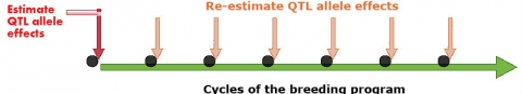
A. Mapping As You Go (MAYG)

The MAYG strategy re-estimates the value of QTL alleles as new germplasm is developed over breeding cycles (Podlich et al., 2004). In general, MAYG involves the following steps:

1. Estimation of QTL effects in progeny of an initial set of crosses.
2. Construction of marker alleles based on information from step 1 for MAS on germplasm.
3. Creation of new set of crosses among selected lines.
4. Update of the estimates of the QTL effects for use in the next selection cycle.
5. Continuation of the process (1-5) using new estimates of QTL effects (Fig. 4).

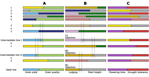
B. Breeding By Design

Markers are useful in development of haplotype maps (see the eModule on Markers and Sequencing). Breeding by design requires information about chromosome haplotypes. Figure 5 below is an example of a haplotype map. Breeding by design describes the use of chromosome haplotypes to aid selection of F₂ or BC individuals to develop superior elite line genotype.

Breeding by design describes the use of chromosome haplotypes to aid selection of F2 or BC individuals to develop superior elite line genotype.

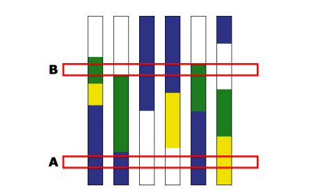
The Principle of Breeding by Design

In Fig. 6, three chromosomes, A, B and C, of five parental lines, 1-5 are indicated side by side. Selection of specific recombination points on chromosomes A and B are done and chromosome C is selected from parental line 1. Dotted lines delineate marker positions used to select for the desired recombinants. The genome composition of the ideal line with respect to the three chromosomes is indicated.

 

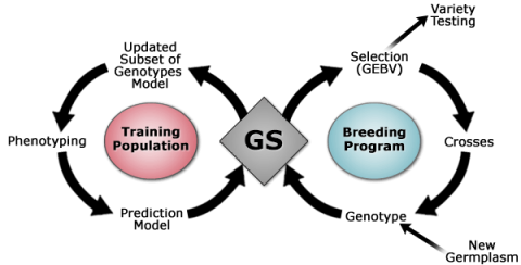
Genomic Selection

Advantage of Using GS

As discussed in previous sections, selection based on the genotype rather than the phenotype may result in faster and more efficient ways to conduct selection. However, the paradox of MAS makes detection of quantitative traits with low heritability less reliable because the power of detecting quantitative trait loci (QTL) depends on size of the mapping population and heritability of the trait. Also, application of MAS in small populations may lead to bias in magnitude of QTL effects and estimation of location of QTL. In contrast, Genomic Selection (GS) is a form of MAS involving estimation of the breeding values of lines in a population by evaluating their phenotypes and scores of markers that span the entire genome. The incorporation of all marker information in the GS prediction models helps avoid biased estimate of marker effects allowing the capturing of variation caused by small-effect QTL.

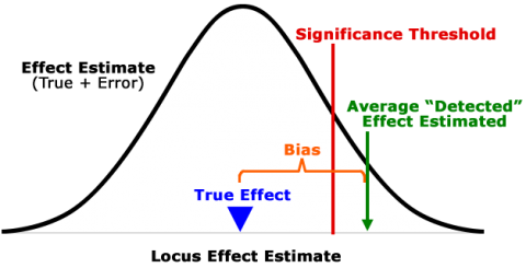
GS Principles

QTL studies detect in most cases only the “tip of the iceberg”, a limited number of QTL representing a small subset of all QTL affecting the trait(s) of interest. As QTL mapping employs a significance test, most true QTL are not detected (below significance threshold) (Fig. 7). Locus effect estimates of QTL that are detected are generally inflated (Fig. 7; “Beavis effect”).

Application of GS

The application of GS in plant breeding was first introduced in the early 2000 (Meuwissen et al., 2001) and is based on the following principles:

1. Dense marker maps covering all chromosomes allow accurate estimation of breeding values of individuals that have no phenotypic record and no progeny.
2. Estimation of breeding value requires large number of marker haplotype effects.
3. Methods that are based on prior distribution of variance associated with each chromosome segment provide more accurate prediction of breeding values.
4. Selection based on genomic estimated breeding value (GEBV) has potential to increase the rate of genetic gain (Fig. 8) when combined with reproductive techniques, for example, doubled-haploids.

Important Factors

In applying GS it is also important that:

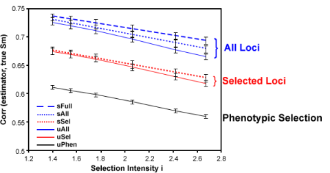
1. All markers contribute to prediction, i.e. there is no distinction between “significant” and “non-significant” effects (Fig. 7). Thus, there is no arbitrary exclusion or inclusion of markers. The value of analyzing all loci is illustrated by Fig. 9.
2. More effects are estimated than there are phenotypic observations.
3. Smaller QTL effects are captured.
4. Genetic relationships are captured.
5. Multiple low cost markers are available.

Two Population Types

In GS, two types of populations are considered:

1. Training population – Both genotypic and phenotypic data should be available allowing fitting of a large number of markers as random effects in a linear model to estimate all marker effects simultaneously. The aim is to capture all of the additive genetic variance caused by alleles with both large and minor effects
2. Breeding population – Only genotypic data are required to allow estimates of marker effects for prediction of breeding values, and selection of lines with GEBV.

GS Methods

The Basic Model

Statistical methods used for GS include, stepwise regression, ridge regression best linear unbiased prediction (RR-BLUP), and Bayesian estimations (Heffner et al., 2009). The basic model (Habier et al., 2007) underlying these methods can be written as:

[latex]y = \mu + \sum_{k}^{} X_{h}\beta _{k}\delta _{k} + e[/latex]

where:
y = a vector of tarit phenotypes
μ = the overall mean
x_k =a column vector of marker genotypes at locus k
β_k = the marker effect
δ_k = a 0/1 ^– indicator variable
e = a vector of random residual effects

Table 3 Characteristics and trends of performance for BLUP and GS methods. Data from Heffner et al., 2009.

Performance with increased
Method	Marker effect; variance assumption	Proportion of markers fitted in model	Marker density	QTL [latex]\dagger[/latex]  density	Large-effect QTL	Small-effect QTL	Inbreeding depression; loss of diversity
Traditional BLUP	N/A	N/A	N/A	N/A	Captured only by phenotype	Captured only by phenotype	Yes
Stepwise regression	Fixed	Subset	Reduced	Reduced	Overestimated	Excluded	Marginally Reduced
RR-BLUP[latex]\ddagger[/latex]	Random; Equal	All	Reduced [latex]\S[/latex]	Increased	Underestimated	Captured	Reduced
BayesA	Random; Unique All>0	All	?	Reduced	More accurately estimated	Captured	Reduced
BayesB	Random; Unique Some=0	All	Insensitive [latex]\S[/latex]	Reduced	More accurately estimated	Captured	Reduced
[latex]\dagger[/latex] QTL, quantitative trait locus. [latex]\ddagger[/latex] RR, ridge regression [latex]\S[/latex] Source: Fernando (2007).

Regression Models

The ability of GS to capture information on genetic relatedness is valuable. However, information on genetic relatedness decays rapidly. Importantly, the amount of information captured is strongly related to the number of markers fitted by a model. In estimating marker effects, two components contribute to an effect, these are, marker and error. When the effect is large, chances are that the error is also large. Thus methods that shrink (regress) the effects toward the mean as of a function of relative error and factor variances are used. Regression models (e.g., Bayesian) can partition contributions of linkage disequilibrium (LD) versus genetic relatedness. Thus regression models help and increase in long-term accuracy in estimating marker effects.

Marker Difference

In GS procedures, marker effects are considered to be random, in contrast to MAS, where marker effects are considered to be fixed effects. The differences between random and fixed marker effects are listed below.

Random markers

• Genome-wide markers
• Each effect considered as coming from a population of marker effects with a probability distribution
• Interested in predicting future values marker effects
• Hypothesis testing may be done on populations, which are considered static
• Estimation and prediction are important
• To predict, one needs to quantify influence of error relative to “factor processes”
• Dependence on population properties best addressed by random effect

Fixed markers

• They are developed from candidate loci
• Each locus is different biologically, i.e., there is no population
• Each candidate locus is a hypothesis
• Hypothesis testing based on effects
• Estimation and prediction are not important
• No particular interest in estimating effects as long as a hypothesis is tested
• Future values of effects are also not relevant.

Simulation Studies

GS vs. MARS Comparison

Simulation studies of testcross performance of doubled haploids in maize (Fig. 10) suggest that GS is more effective than MARS for complex traits under the control of many QTL with low heritability (Table 10). However, GS is less beneficial for recurrent selection for choosing parents of breeding populations or selection of single-crosses (Bernardo and Yu, 2007).

Responses to Different Selections

Table 4 Responses to phenotypic, marker-assisted, and genomewide selection among maize doubled haploids. Relative efficiencies of MAS and GS are highlighted. Data from Bernardo and Yu, 2007.

Heritability
Number of QTL	Method	Number of Markers	0.20	0.50	0.80
20, 40, or 100	Phenotypic selection	0	1.60	2.26	2.61
20	MARS	32	2.50 (0.4)	3.14 (0.4)	3.38 (0.4)
64	2.72 (0.3)	3.42 (0.4)	3.73 (0.4)
128	2.54 (0.3)	3.47 (0.2)	3.87 (0.4)
256	2.26 (0.2)	3.19 (0.2)	3.72 (0.2)
Genomewide selection	64	2.86	3.50	3.76
128	2.98	3.67	4.02
256	3.06	3.72	3.98
512	3.05	3.68	4.10
768	3.06	3.73	4.05
RGS:MARS¶	113%	107%	106%
R(GS-PS):(MARS-PS)#	130%	121%	118%

MAS Compared to GS

The similarities and differences between MAS and GS are shown in Figure 11. In general, MAS involves identification of alleles for development of markers for use in pre-selection of individuals containing an allele of interest. In contrast, GS does not require identification of genes as a source of markers for pre-selection of segregants with desirable alleles. Instead, whole chromosome segments are scanned to estimate the effect of QTL on a trait of interest.

References

Asoro, F. G., M. A. Newell, W. D. Beavis, M. P. Scott, and J-L. Jannick. 2011. Accuracy and Training population design for genomic
selection on quantitative traits in elite North American oats. Plant Genome 4: 132-144.

Bernardo, R. 2002. Breeding for quantitative traits in plants. Stemma Press, Woodburry.

Bernardo, R. 2008. Molecular Markers and Selection for Complex Traits in Plants: Learning from the Last 20 Years. Crop Sci.
48:1649-1664.

Bertrand, C. Y. C., and D. J. Mackill. 2008. Marker-assisted selection: an approach for precision plant breeding in the twenty-first century.
Phil. Trans. R. Soc. B 363:557-572.

Bernardo, R., J. Yu. Prospects for genomewide selection for quantitative traits in maize. Crop Sci. 47: 1082-1090.

Bonnett, D.G., G.J. Rebetzke, and W. Spielmeyer. 2005. Stratehgies for efficient implementation of molecular markers in wheat breeding. Mol. Breeding 15: 75-85.

Cregan, P. B., J. Mudge, E. W. Fickus, D. Danesh, R. Denny, and N. D. Young. 1999. Two simple sequence repeat markers to select for
soyben cyst nematode resistance conditioned by the rhg1 locus. Theor Appl Genet 99: 811-818.

Eagles, H.A., H. S. Bariana, F. C. Ogbonnaya, G. J. Rebetzke, G. J. Hollamby, R. J. Henry, P. H. Henschke, and M. Carter. 2001.
Implementation of markers in Australian wheat breeding. Aust. J. Agric. Res. 52: 1349-1356.

Eathington, S. R., T. M. Crosbie, M. D. Edwards, R. S. Reiter, and J. K. Bull. 2007. Molecular markers in a commercial breeding program.
Crop Sci. 47(S3):S154-S163.

Habier, D., R. L. Fernando, and J. C. M. Dekkers. 2007. The impact of genetic relationship information on genome-assisted breeding values.
Genetics 177:2389-2397.

Heffner, E. L., M. E. Sorrells, and J-L. Jannick. 2009. Genomic selection for crop improvement. Crop Sci 49: 1-12.

Hospital, F. 2009. Challenges from effective marker-assisted selection in plants. Genetics 136:303-310.

Lande, R., and R. Thompson. 1990. Efficiency of marker-assisted selection in the improvement of quantitative traits. Genetics 124:743-756.

Meuwissen, T. H. E., B. J. Hayes, and M. E. Goddard. 2001. Prediction of total genetic value using genome-wide dense marker maps. Genetics
157: 1819-1829.

Moreau, L., A. Charcosset, F. Hospital, and A. Gallais. 1998. Marker-assisted selection efficiency in populations of finite size. Genetics
148:1353-1365.

Moreau, L., S. Lemarié, A. Charcosset, and A. Gallais. 2000. Economic efficiency of one cycle of marker-assisted selection. Crop Sci.
40:329-337.

Nakaya, A., and S. N. Isobe. 2012. Will genomic selection be a practical method for plant breeding? Annal. Bot. 110. 1303-1316.

Peleman, J. D., and J. R. van der Voort. 2003. Breeding by design. Trend Plant Sci. 8: 330-334.

Piepho, H. P., J. Möhring., A. E. Melchinger, and A. Büchse. BLUP for phenotypic selection in plant breeding and variety testing. Euphytica. 161: 209-228.

Podlich, D. W., C. R. Winkler, and M. Cooper. 2004. Mapping As You Go: An effective approach for marker-assisted selection of complex traits. Crop Sci. 44: 1560-1571.

Reyna, N., and C. H. Sneller. 2001. Evaluation of marker-assisted introgression of yield QTL alleles into adapted soybean. Crop Sci. 41: 1317-1321.

Tanksley, S. D., and C. M. Rick. 1980. Isozymic gene linkage map of the tomato: Applications in genetics and breeding. Theor. Appl. Genet. 57: 161-170.

Utz, H.F., and A.E. Melchinger. 1994. Comparison of different approaches to interval mapping of quantitative trait loci. In: Ooijen, J.W. van, and J. Jansen (eds.), Biometrics in Plant Breeding: Applications of Molecular Markers. Wageningen, 195-204.

Yousef, G. G., and J. A. Juvik. 2001. Comparison of phenotyoic and marker-assisted selection for quantitative traits in sweet cor. Crop Sci. 41: 645-655.

Zhong, Shengqiang, and Jannink, Jean-Luc. 2007. Using QTL results to discriminate among crosses based on their progeny mean and variance. Genetics 177(1): 567-576.