
Chapter 8: Genome Construction
Thomas Lübberstedt; Walter Suza; and William Beavis
One of the main challenges in plant breeding is the development of the best marker-assisted breeding method for complex traits. At the present, marker-based approaches are limited in their ability to detect and quantify marker-trait relationships, in particular for traits that are under the influence of gene x gene and gene x environment interactions. Also, as you have learned in previous lessons of this course, QTL estimates are biased by population size and a limited set of environments, making QTL estimates less suitable for crop improvement. For this reason, simulation modeling is an emerging important tool to choose among proposed breeding methods because experimental evaluation of breeding methods is time and resource-limited. Another challenge is management of multiple breeding objectives for several complex traits, making it more likely that an operations research approach called multi-objective optimization will gain favor in crop breeding. Thus, this lesson will introduce operations research as a tool to address multiple crop breeding objectives.
- Summarize and state the concept of genetic gain
- Introduce the concept of multi-objective optimization
- Introduce the concept of operations research in plant breeding
Recapitulation of the Concept of Genetic Gain
Definition
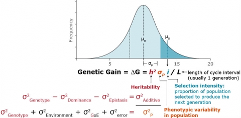
Genetic gain (∆G) is defined as the predicted change in the mean value of a trait within a population as a result of selection. The ∆G equation (Fig. 3) allows the comparison of predicted effectiveness of particular breeding methods and helps breeders decide how resources should be allocated for achieving various breeding objectives.
Commercialization Challenges
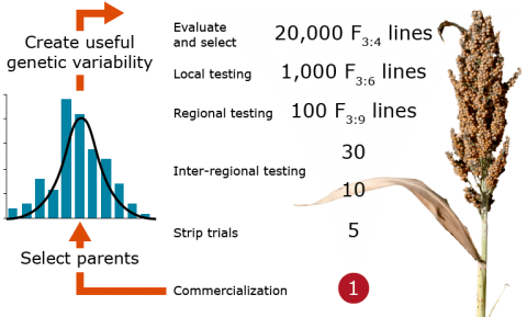
Figure 4 illustrates a generic plant breeding program involving mating, evaluation, selection, and testing of breeding materials resulting in commercialization of a cultivar. Such a program faces the challenges of time to commercialization of a cultivar, and resources allocated to obtain such cultivar from thousands of individuals.
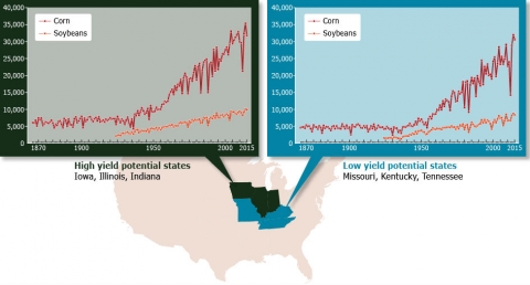
Crop Yield Progress
Despite such challenges, from the 1940s, the yields of corn and soybean in the United States have continued to rise (Fig. 5) mainly due to improvement in crop genetics and agronomic practices.
Global Food Demand Trends
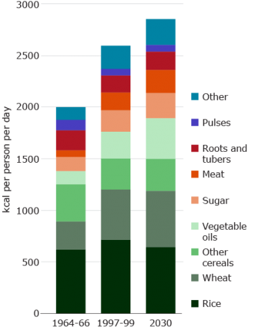
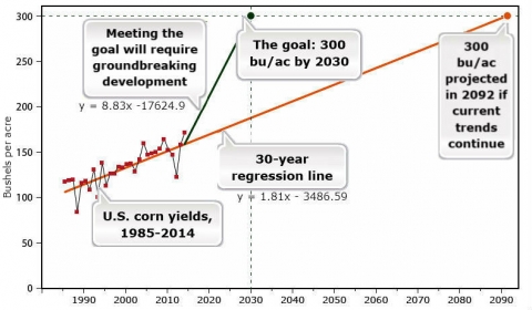
Despite the upward trend in crop yields in the US and other parts of the world, rising human and animal populations will pose a greater demand for more to be produced per unit of land. The growing global demand for food (Fig. 6) raises the question of whether it is possible to double the current level of production in the next 20 years (Fig. 7). Undoubtedly, to reach 300 bushels/acre of corn by 2030 will require cutting-edge approaches in genomics and breeding. But the problem will be the cost of reaching such a high level of yield with limited time and resources. Thus, integration of new approaches, for example, Genomic Selection, transgenics, and operations research, may be necessary. The next lesson sections entail application of operations research tools in plant breeding as a novel approach to increase ∆G.
Need for Advancement
Historically plant breeding has been a form of art: to create new varieties. Thus, ∆G has depended on management of resources, to produce new varieties; while optimization has been ignored. Nonetheless, plant breeding has the potential to become an engineering discipline, relying on operations research, which will be necessary for average yields to double by 2030 (Fig. 7).
Multi-Objective Optimization
Introduction
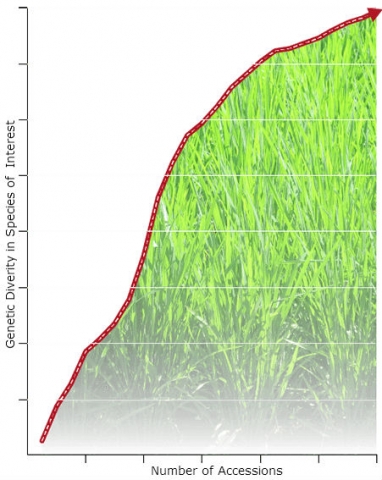
Multi-objective optimization (MO) is an operations research approach used in various fields, including engineering, finance, biomedicine and management. Optimization involves application of more than one objective processes for evaluation that can take into account multiple criteria that need to be considered for making a decision. Therefore, as information on plant genomes continue to emerge, it is now possible to apply the MO approach for large scale plant breeding (Xu et al., 2011). For example, a plant breeding goal may have two objectives, 1) selection and fixation of desirable genes at a set of loci controlling a trait of interest, and 2) keeping genetic variability at the remaining loci to retain adaptability. The challenge of applying MO to solve these competing objectives is identification of optimal solutions to the problems (Chinchuluun and Pardalos, 2007). Such solutions are called Pareto optimal solutions, and they are a measure of MO optimization efficiency.
Pareto optimal solutions
We will not dwell on the mathematics used to derive Pareto optimal solutions in this lesson. But it is important to know that there usually exist multiple Pareto optimal solutions for MO problems, and searching for all Pareto optimal solutions can be expensive and time consuming (Chinchuluun and Pardalos, 2007). Nonetheless, recent advances in computational research suggest that it is possible to obtain Pareto optimal solutions for plant breeding problems within reasonable computation time (Xu et al., 2011). Such solutions will be useful tools to help plant breeders make informed decisions in the world of large amounts of genomics data for multiple breeding objectives for complex traits. 2011). Such solutions will be useful tools to help plant breeders make informed decisions in the world of large amounts of genomics data for multiple breeding objectives for complex traits.

Operations Research in Plant Breeding
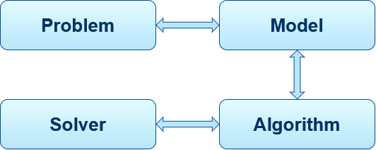
Operations Research involves the application of mathematical models to provide optimal solutions to a problem. An OR approach (Fig. 10) consists four components, 1) Problem, 2), Model, 3) Algorithm, and 4) Solver.
Step 1: Defining the Problem
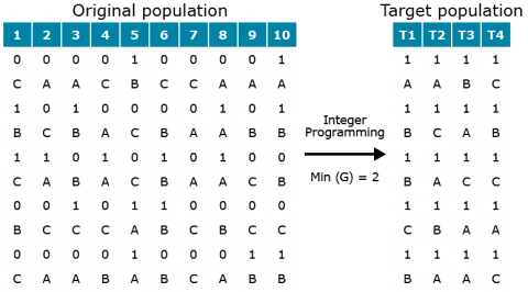
There is an original population of individuals (Fig. 11). Each individual has a pair of chromosomes, and each chromosome has a number of genes. Some genes are undesirable, while the desirable ones have different variants. The desirable genes will be assigned a value of 1 and undesirable 0. What is the best way to assemble all variants of desirable genes into a target population?
Step 2: Developing a Model
A model has four key elements – data, decisions, objective, and constraints.
- Data
- Decisions – A decision would have to be made about number of data and recombination points, and number of chromosomes in the target population.
- Objective – The objective is to maximize probability of getting the target population.
- Constraints – Constraints can be, for example, the number of chromosomes in target population without undesirable alleles, but such that all desirable variants are retained. Also, the maximum number of recombination events could be another constraint.
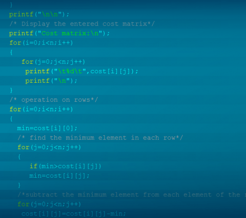
Step 3: Designing a Suitable Algorithm
The problem in this example belongs to a class of so-called non-deterministic polynomial-time hard (NP-hard) problems (Xu et al. 2011). Importantly, if an algorithm solves one NP-hard problem, it can be used to solve all other NP-hard problems.
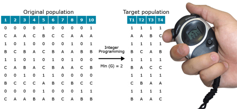
Step 4: Solving the Problem
Computation time spent to solve the problem in Figure 11 was 0.03 seconds (W.D. Beavis, personal communication).
Genome Construction vs. Genomic Selection
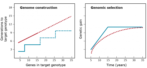
The hypothesis is that genome construction is better than genomic selection (Fig. 13). The hypothesis is developed from the premise that a target genotype can be defined. However, if the target genotype has to be determined using experimental methods, then GS will be more effective because experimental methods are underpowered and biased.
References
Chinchuluun, A. P. M. Pardalos. 2007. A survey of recent developments in multiobjective optimization. Ann. Oper. Res. 154: 29-50.
Egli, D. B. 2008. Comparison of corn and soybean yields in the United States: Historical trends and future prospects. Agron J. 100: S-79-S-88.
Expert Meeting on “How to Feed the World in 2050,” FAO, Rome, 24-26 June 2009.
FAO, 2002. World agriculture: towards 2015/2030. United Nations, 2002.
Moose, S. P., and R. H. Mumm. 2008. Molecular plant breeding as the foundation for 21st century crop improvement. Plant Physiol. 147: 969-977.
Xu, P., L. Wang, and W. D. Beavis. 2011. An optimization approach to gene stacking. Europ. J. Oper. Res. 214: 168-178.
