
Chapter 5: Categorical Data Multivariate
Ron Mowers; Kendra Meade; William Beavis; Laura Merrick; Anthony Assibi Mahama; and Walter Suza
In the previous chapter, we saw examples of data from the binomial distribution, in which there are two categories for classification. In there, we develop a method for categorical data that occur in multiple categories. Discrete distributions which can have more than two categories (Fig. 1) are referred to as multinomial distributions, and their analyses often employ the Chi-squared, [latex]\chi^2[/latex], method.
- Understand how to use the [latex]\chi^2[/latex] test to evaluate discrete distributions of data.
- Be able to categorize data using contingency tables.
- Learn how to conduct statistical tests of differences among proportions, of independence, and of heterogeneity of discrete data sets.
Chi-Square Testing
Chi-square ([latex]\chi^2[/latex]) tests may be used to analyze counts in categorical data. Counts of data or data categorized on the basis of qualitative characteristics may be evaluated for significant differences using the chi-square test.
For example, during a recent growing season, 17 days had precipitation of 0-10mm, 9 days had precipitation of 10-20mm, 6 days had precipitation of 20-30mm, and 5 days had greater than 30mm of rain. Individually, these data may not be of much use. But using the chi-square test, you can determine if this distribution is significantly different from that expected based on the historical record.
A question you might ask would be: Did we have more days of heavier rain (> 30mm) or fewer days of light rain (0-10mm)? Often this is a more meaningful way of classifying rainfall than total rainfall during a season.
Evaluation
Such data need to be evaluated to determine if differences in counts of the data are significant. Analyses of such data are done as analyses of counts. The test often applied to these is the [latex]\chi^2[/latex] test.
[latex]\chi^2[/latex] may be thought of as the combined deviation of multiple counts from their expected values. The [latex]\chi^2[/latex] distribution is itself a continuous distribution, taking on many different shapes depending on the degrees of freedom as depicted by Figure 2.
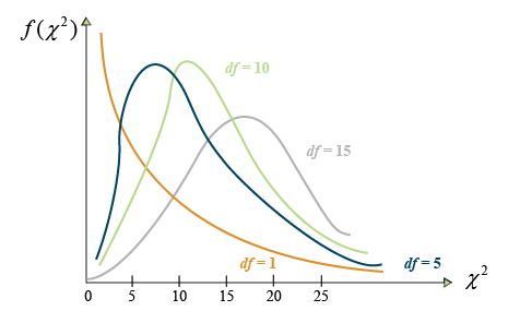
In Figure 2, the number on the Y-axis is the probability that the[latex]\chi^2[/latex] value indicated on the X-axis occurs. The probability of significance is determined by the area under the graph, usually to the right of a certain number. For example, the probability of a [latex]\chi^2[/latex] value of 25 or larger of occurring.
Notice that as the number of df becomes larger, the [latex]\chi^2[/latex] distribution more closely approaches the normal distribution to which it is related. At lower degrees of freedom, the [latex]\chi^2[/latex] distribution is skewed, with lower values having a higher probability of occurrence. At higher degrees of freedom (>15), the distribution closely approximates a normal distribution.
Formula
The chi-square method performs the analysis using counts. It estimates the difference in the observed number counted from the number expected. The value of the test on the χ2 distribution is determined by its closeness to the expected values.
[latex]\chi^2=\sum{\frac{(observed-expected)^2}{expected}}[/latex]
[latex]\text{Equation 1}[/latex] Formula for computing chi-square value.
The summed terms comprise a [latex]\chi^2[/latex] value which occurs somewhere on the graph.
The farther to the right on the graph the value occurs, the more the data deviate from expected. A critical value is determined for a given probability level (Fig. 2).
Evaluating Hypotheses
For a significance level of 0.05, a [latex]\chi^2[/latex] value to the right of the critical [latex]\chi^2[/latex] value would have a 5% chance of occurring. Thus, the [latex]\chi^2[/latex] test would be significant at the 0.05 level. The interpretation is that the data deviated enough from expected to produce the large [latex]\chi^2[/latex] value in the analysis. Data to the left of critical [latex]\chi^2[/latex] value line are not significant (Fig. 3).
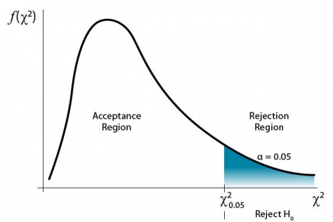
This is based on a null hypothesis that the observed data occur as expected. The alternate hypothesis would be that the data deviate from the expected values.
Yates’ Correction
Small numbers of counts should be avoided if possible, as well as situations with few degrees of freedom. In these cases, the power of the test is low and the chi-square approximation to the true distribution probabilities may be inaccurate. Notice how the curves above change from having a few degrees of freedom to many degrees of freedom. When possible, it is recommended to have each category contain at least five data points. In situations where you have one df, such as 2 x 2 contingency table, you should apply Yates’ Correction for Continuity. This correction factor involves subtracting 0.5 from the absolute value of each category or cell:
Yates’ correction for continuity:
[latex]\chi^2=\sum{\frac{(|observed-expected|-0.5)^2}{expected}}[/latex]
[latex]\text{Equation 2}[/latex] Formula for Yates’ correction for continuity.
The two straight vertical lines around “observed-expected,” i.e. ‘||’, mean that you should use the absolute value of that difference — you should convert any negative values to positive before subtracting 0.5.
Testing Proportions
Hypotheses
Let’s look at a simple example. A plant breeder is examining the inheritance of chlorophyll in a new maize cultivar. It is hypothesized that three of every four (3:1 ratio) plants of the new population will be colored green while the others will be yellow. After conducting an emergence test, it is found that of 200 plants emerged, the ratio of green to yellow is 1:1, 100 green:100 yellow. Is this result different from what was expected? At what probability level is it significant?
The [latex]\chi^2[/latex] test will be used to test this example. We begin with the hypothesis:
- [latex]H_{0}[/latex]: The ratio of green to yellow in the emerged plants is the same as expected.
- [latex]H_{\alpha}[/latex]: The ratio of green to yellow in the emerged plants is different from expected
- [latex]\alpha = 0.05[/latex]
Calculation
The method of testing here divides the total emerged plants into their expected numbers. Of 200 plants it is found that 100 were green and 100 yellow. Compare this to the expected numbers. In the 3:1 expected ratio, 150 would be expected to be green and 50 expected to be yellow. You have the data necessary to calculate the [latex]\chi^2[/latex] statistic. Basically, there are two different cells or observations, the number of green and the number of yellow plants. We know the expected value of each. Use the [latex]\chi^2[/latex] formula to sum the differences over the two categories.
Since there are two observations and we are constraining the observations by one, the df are 2 – 1 = 1. We use the Yates correction for continuity accordingly and subtract 0.5 from the absolute difference for each category. An example is below.
[latex]\chi^2=\sum{\frac{(|observed-expected|-0.5)^2}{expected}}[/latex]
[latex]\chi^2=\sum{\frac{(|100-150|-0.5)^2}{150}} + {\frac{(|100-50|-0.5)^2}{50}}[/latex]
[latex]\chi^2=\frac{(49.5)^2}{150} + \frac{(49.5)^2}{50} = \frac{(2450.25)}{150} + \frac{(2450.25)}{50}[/latex]
[latex]\chi^2=\text {16.335 + 49.005 = 65.34}[/latex]
[latex]\chi^2= 65.34 \text { with 1 df}[/latex]
[latex]\chi^2 \text{@ alpha = 0.05 and 1 df is 3.84}[/latex]
[latex]\chi^2 \text{ is therefore significant}[/latex].
The [latex]\chi^2[/latex] significance value at 0.05 is 3.84. Even at a significance level of 0.001, the critical [latex]\chi^2[/latex] value is 10.827. What is observed is very different from what was expected. The testing indicates the null hypothesis IS NOT correct. We would reject the null hypothesis, i.e., the ratio of green to yellow plants is different from expected.
Note that the binomial distribution provides an exact test, which is better than the [latex]\chi^2[/latex] test, even with the Yates’ correction (subtracting the 0.5 in the formula).
Calculating a Chi-Square Test (1)
The discussion of the [latex]\chi^2[/latex] test has introduced several interpretations of the test. Its main premise is to test a set of counts, cells, or categories to determine if the numbers in each are significantly different from the numbers expected in each situation.
In this exercise, we will perform the calculation on the original simple [latex]\chi^2[/latex] test (without Yates’ correction). In an emergence test of 200 plants, 100 were observed to be green, while 100 were found to be yellow (a 1:1 ratio). The expected ratio was 3:1 (150 green to 50 yellow in this case). Are the observed numbers different enough to be significant? In other words, test the hypothesis:
H0: The true ratio is 3 green : 1 yellow
HA: The true ratio is not 3 green : 1 yellow
Steps
Enter the data in Excel to get this table.
| Color | Count |
| Green | 100 |
| Yellow | 100 |
| Total | =SUM(B2:B3) |
The expected counts are 150 green and 50 yellow. The expected counts can be calculated from the total observations and the 3:1 ratio. If the expected ratio is 3:1 there are 4 total.
| Color | Count | Expected Ratio |
| Green | 100 | 3 |
| Yellow | 100 | 1 |
| Total | 200 | =SUM(C2:C3) |
Divide both sides of the ratio by 4 to get a ratio with a total of 1.
| Color | Count | Expected Ratio | Normalized Ratio |
| Green | 100 | 3 | =C2/C4 |
| Yellow | 100 | 1 | =C3/C4 |
| Total | 200 | 4 | =SUM(D2:D3) |
The expected counts can then be calculated by multiplying the total number of observations by the expected ratio.
| Color | Count | Expected Ratio | Normalized Ratio | Expected Count |
| Green | 100 | 3 | 0.75 | =D2*B4 |
| Yellow | 100 | 1 | 0.25 | =D3*B4 |
| Total | 200 | 4 | 1 | =SUM(E2:E3) |
Check your math by making sure that the expected counts sum to the same number as the observed counts.
| Color | Count | Expected Ratio | Normalized Ratio | Expected Count |
| Green | 100 | 3 | 0.75 | 150 |
| Yellow | 100 | 1 | 0.25 | 50 |
| Total | 200 | 4 | 1 | 200 |
The [latex]\chi^2[/latex] statistic is calculated using the observed and expected counts. There are two categories in this problem: green and yellow. Within each category, calculate ((O – E)2/ E) where O is an observed count and E is an expected count, then sum across the categories to find the statistic.
| Color | Count | Expected Ratio | Normalized Ratio | Expected Count | Chi-Squared |
| Green | 100 | 3 | 0.75 | 150 | =((B2-E2)^2)/E2) |
| Yellow | 100 | 1 | 0.25 | 50 | =((B3-E3)^2)/E3) |
| Total | 200 | 4 | 1 | 200 | =SUM(F2:F3) |
| Color | Count | Expected Ratio | Normalized Ratio | Expected Count | Chi-Squared |
| Green | 100 | 3 | 0.75 | 150 | 16.66666667 |
| Yellow | 100 | 1 | 0.25 | 50 | 50 |
| Total | 200 | 4 | 1 | 200 | 66.66666667 |
Find the degrees of freedom for this test by subtracting one from the number of rows. There are two rows, so there is one degree of freedom.
The p-value for this test can be found using the formula “CHISQ.DIST.RT(Chi, DF)”. Enter the calculated chi-squared statistic for Chi and the correct degrees of freedom.
| Chi-Squared | =F4 | 66.66666667 |
|---|---|---|
| Deg. of Freedom | 1 | 1 |
| p-value | =CHISQ.DIST.RT(C8,C9) | 3.21526E-16 |
A p-value less than 0.05 means that the test is significant. In this case, the p-value is very small. This means that the test is highly significant, and there is little or no chance that the results would have occurred by chance, and the null hypothesis should be rejected.
Testing a 9:3:3:1 genetic ratio
We use the same principles as in the first exercise to check other genetic ratios. Use Excel to analyze the data from Example 18.10 on page 282 in our textbook. We observe 150, 42, 50, and 8 in classes A, B, C, and D, respectively. From genetic theory, we hypothesize a 9:3:3:1 ratio. Should we reject this hypothesis?
- H0: The true ratio is 9A : 3B : 3C : 1D
- HA: The true ratio is not 9A : 3B : 3C : 1D
Open a new Excel workbook and enter this data set:
| Class | Count |
|---|---|
| A | 150 |
| B | 42 |
| C | 50 |
| D | 8 |
Follow the same steps used in Exercise 5.1. The ratio for this hypothesis is 9:3:3:1, with a total of 16. This ratio is used to calculate the expected counts.
| Class | Count | Expected Ratio | Normalized Ratio | Expected Count | Chi-Squared |
|---|---|---|---|---|---|
| A | 150 | 9 | 0.5625 | 140.625 | 0.625 |
| B | 42 | 3 | 0.1875 | 46.875 | 0.507 |
| C | 50 | 3 | 0.1875 | 46.875 | 0.2083333333 |
| D | 8 | 1 | 0.0625 | 15.625 | 3.721 |
| Total | 250 | 16 | 1 | 250 | 5.0613333333 |
| Chi-Squared | 5.0613333333 |
|---|---|
| Deg. of Freedom | 3 |
| p-value | 0.1674 |
The probability of a greater [latex]\chi^2[/latex] (the p-value) is 0.1674, and we fail to reject the null hypothesis. This can be determined from the p-value, which is greater than the alpha level of 0.05.
Observations vs. Expectations
To test whether an observed proportion is different from the theoretical proportion. A proportion measures what percentage of a population that has a certain characteristic or does not have a certain characteristic. These are measured as a proportion or percentage of the population (35% of the population will have a trait) or as ratios (3:1) ratio means 3 of every four members of a population contain a genetic allele) within the population. When sampling a population, you may want to know whether this sample population has a characteristic occurring in a different proportion as compared to the whole population. Or an experimental treatment may cause a population to have a different ratio of occurrence of a certain characteristic than expected. Did what happened in an experiment deviate from what was expected? How much did it deviate? These are questions which can be answered using the [latex]\chi^2[/latex] test.
We have already seen some proportion data in the binomial distribution in chapter 3 on Categorical Data—Binary. The chi-square analyses for the simple case of two categories agree with the results of the normal approximation to the binomial. However, the [latex]\chi^2[/latex] can be used for counts from more than just two categories.
Contingency Tables
Contingency tables are tables of count data and can be analyzed with [latex]\chi^2[/latex]. The simple proportion example shown earlier could have been analyzed with a contingency table. Often more complex experiments have interactions between two ways of categorizing the data. For example, flower color and leaf pubescence. The contingency table simplifies the comparison by breaking down the categories for each variant into a table format, which is designed for completing two-way analyses. It has a form that classifies the first set of data over the columns and the second set over the rows (Table 1).
| Level | 1 | 2 | 3 | 4 | n/a | c | Total |
|---|---|---|---|---|---|---|---|
| 1 | O11 | O12 | O13 | O14 | n/a | O1c | r1 |
| 2 | O21 | O22 | O23 | O24 | n/a | O2c | r2 |
| 3 | O31 | O32 | O33 | O34 | n/a | O3c | r3 |
| n/a | n/a | n/a | n/a | n/a | n/a | n/a | n/a |
| n/a | n/a | n/a | n/a | n/a | n/a | n/a | n/a |
| n/a | n/a | n/a | n/a | n/a | n/a | n/a | n/a |
| r | Or1 | Or2 | Or3 | Or4 | n/a | Orc | rk |
| Total | c1 | c2 | c3 | c4 | n/a | cm | n |
Notice that each row and column have a total, rk and cm, respectively. These numbers are the counts for each cell defined by the row category and column category. Comparing these numbers to the total of the whole table establishes the total proportion break-down of each cell. The row totals give a breakdown of the row categories and the column totals for the column categories. Summing each of the row totals and column totals produces the grand total. The row and column totals are also integral to the [latex]\chi^2[/latex] test because they can be used to calculate an expected value in each cell for a two-way analysis. This expected value is then compared with the actual number counted by using the [latex]\chi^2[/latex] test.
Expected Values
The expected value calculation assumes independence of the two criteria (which will be tested in the next section). This assumption states that the variables in the columns and the rows have no interaction; they are independent of each other. One property of independence is that the expected value of each cell should be the product of the row and column category proportions times total number. This results in the following formula (Equation 3):
[latex]\text{cell expected value} = \dfrac{\text{(row total) x (column total)}}{\text{grand total}}[/latex].
[latex]\text{Equation 3}[/latex] Formula for computing expected values of cells in table.
The number calculated uses the relative proportion of each row and column to calculate the number each cell should contain. The calculation of the [latex]\chi^2[/latex] occurs by summing the deviations of each cell from its expected value.
Degrees of Freedom
The degrees of freedom associated with this are calculated as the product of one less than the row and column categories.
[latex]\text{degrees of freedom}={\text{(number of rows - 1) x (number of columns - 1)}}[/latex]
[latex]\text{Equation 4}[/latex] Formula for computing degrees of freedom.
For example, a 2 x 2 table would have (2-1) x (2-1) = 1 df.
For better statistical inferences, each cell should contain at least a count of five. If smaller counts occur, combining of row or column categories is suggested to create cell counts larger than five. Recent studies suggest that even though the observed count in a cell is five, the expected count for cells need only be larger than six when significance at the 0.05 level is needed or an expected value larger than 10 when significance at the 0.01 level is desired.
The simplest case of contingency tables is a 2 x 2 analysis. But more detailed tables may be created, even into multiple dimensions. When using a 2 x 2 table, the correction for continuity should be used. Other corrections than Yates’ Correction for Continuity exist for other situations.
Test for Independence
Two-way Example
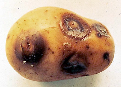
An example of this is the effect of different fertilizer treatments on the incidence of blackleg (Bacterium phytotherum) on numbers of potato seedlings and tubers (Fig. 4).
Our objective is to test whether the occurrence of the disease has some relationship to nitrogen or manure fertilizer application.
The null hypothesis is that fertilizer and Blackleg occurrence have no relationship, i.e., fertilizer application and Blackleg are independent. Data are contained in Table 2.
We then compute a [latex]\chi^2[/latex] statistic to see if the value is high enough to reject the null.
| Observed frequencies | Blackleg | No blackleg | Total |
|---|---|---|---|
| No fertilizer | 16 | 85 | 101 |
| Nitrogen only | 10 | 85 | 95 |
| Manure only | 4 | 109 | 113 |
| Nitrogen and manure | 14 | 127 | 141 |
| Total | 44 | 406 | 450 |
Blackleg Example
These observed values (Table 2) are compared to the calculated expected values using the expected value equation (Equation 3) and set up in an expected value table (Table 3).
| Expected frequencies | Blackleg | No blackleg | Total |
|---|---|---|---|
| No fertilizer | 9.9 | 91.1 | 101 |
| Nitrogen only | 9.3 | 85.7 | 95 |
| Manure only | 11.0 | 102.0 | 113 |
| Nitrogen and manure | 13.8 | 127.2 | 141 |
| Total | 44 | 406 | 450 |
The computed [latex]\chi^2[/latex] values for each cell using Equation 1 are shown in Table 4.
| [latex]\frac{\textrm{(Observed - expected)}^2}{\textrm{expected}}[/latex] | Blackleg | No blackleg |
|---|---|---|
| No fertilizer | 3.76 | 0.41 |
| Nitrogen only | 0.05 | 0.01 |
| Manure only | 4.45 | 0.48 |
| Nitrogen and manure | 0.00 | 0.00 |
| Total | 8.26 | 0.90 |
Calculating Differences
The calculated [latex]\chi^2[/latex] from summing over the table values is 9.16. This is larger than the significance value at the 0.05 level (3 df), 7.82. The degrees of freedom are (4–1)(2–1) = 3 because there are 4 rows and 2 columns. The deviations from expected in the cells are large. The expected value in each cell assumes independence of the conditions. Since the data deviate from those values significantly, we reject the null hypothesis of independence and conclude that the fertilizer treatment affected the incidence of blackleg in this experiment.
Testing for Independence of Data
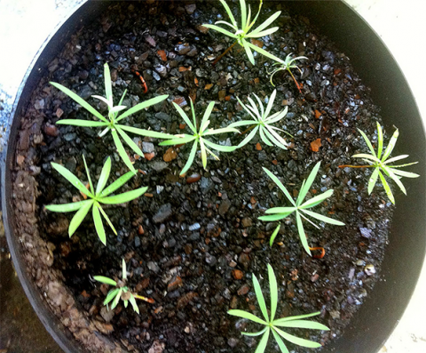
We will duplicate the analysis of independence of data sets using the text example 18.13 with Excel. Five storage methods were tested for effects on the germination of peas (Fig. 5). The data are from Table 18.5 in Practical Statistics and Experimental Design for Plant and Crop Science.
First, enter data into an Excel table with the variables ‘Germinated’ (Yes or No) and ‘Count’. Your data should look like in Table 5.
| Storage Method | Germinated | Count |
|---|---|---|
| A | yes | 112 |
| A | no | 12 |
| B | yes | 76 |
| B | no | 14 |
| C | yes | 88 |
| C | no | 32 |
| D | yes | 43 |
| D | no | 7 |
| E | yes | 92 |
| E | no | 8 |
The hypothesis tested here is:
- H0: Germination and Storage method are independent of each other
- HA: Germination and storage method are not independent of each other
Testing for Independence of Data (2)
Make the analysis easier by arranging the data into a table.
Sum across each column and row. Then sum the column or row totals to find the grand total. This is a good chance to check the arithmetic by making sure that the column totals and row totals sum to the same value (Table 6).
| Observed | A | B | C | D | E | Row Total |
| Yes | 112 | 76 | 88 | 43 | 92 | 411 |
| No | 12 | 14 | 32 | 7 | 8 | 73 |
| Column Total | 124 | 90 | 120 | 50 | 100 | n/a |
| Grand Total | n/a | n/a | n/a | n/a | n/a | 484 |
The expected counts can now be calculated using row, column, and grand total. Each expected count is calculated using the formula (Equation 5):
[latex]{\dfrac{\text{(Col. Total x Row Total)}}{\text{Grand Total}}}[/latex]
[latex]\text{Equation 5}[/latex] Formula for computing expected counts.
The expected values have been filled into Table 7. See if you can repeat the results in your own table.
| Observed | A | B | C | D | E | Row Total |
| Yes | 105.2975207 | 76.42561983 | 101.9008264 | 42.45867769 | 84.91735537 | 411 |
| No | 18.70247934 | 13.57438017 | 18.09917355 | 7.541322314 | 15.08264463 | 73 |
| Column Total | 124 | 90 | 120 | 50 | 100 | n/a |
| Grand Total | n/a | n/a | n/a | n/a | n/a | 484 |
We see that the Pearson [latex]\chi^2[/latex], computed from data in Table 8, is 19.379 (Table 9), and we, therefore, reject the hypothesis that storage methods are independent of germination. The degrees of freedom can be calculated as: (Rows – 1) * (Columns – 1). The p-value is less than 0.05, so we reject the null hypothesis.
| [latex]\chi^2[/latex] | A | B | C | D | E |
| Yes | 0.426631406 | 0.002370308 | 1.896284678 | 0.00690153 | 0.59073767 |
| No | 2.401993258 | 0.013345158 | 10.6763425 | 0.038856561 | 3.325932299 |
| Column Total | 2.828624664 | 0.015715465 | 12.57262718 | 0.045758091 | 3.916669666 |
| Total | 19.37939507 |
|---|---|
| DF=(r-1)*(c-1) | 4 |
| p-value | 0.000661886 |
Testing for Independence of Data (3)
The test was for independence here. Independence would mean that the two categories have no effect on each other. The observed cell values, if independent, would not deviate much from the expected values. In this case, the data have deviated enough to be significant at the 0.001 level. Our conclusion then is that there is some effect of storage method on the viability of plants.
Two-way Contingency Tables
We can test to see if two categorical variables are associated. The contingency table is applied in situations where we have a two–way (or higher) classification structure. We may wish to test to see if the two different bases for categories are independent of each other. For example, we might want to learn if two transgenes are segregating independently or if they are linked. In fact, the null–hypothesis assumption in calculating the expected values of cells assumes independence of the two categorizations. The two–way analysis sorts the data to compare the interaction between variables. If the data are independent, then the numbers in the cells should be similar to the expected values. If the data are not independent, or there is a significant amount of interaction between variables, the contingency table and [latex]\chi^2[/latex] test will indicate numbers different from expected in the cells.
The [latex]\chi^2[/latex] statistic can be applied to test for independence. The calculation is done as illustrated previously. The squared differences between the observed and expected, divided by expected, are summed over all cells of the table and tested via the [latex]\chi^2[/latex] statistic.
Test for Heterogeneity
We also can test whether several samples are homogeneous enough to be pooled together. The test for heterogeneity is similar in method to the test for independence, which tests each cell for its difference from expected. But interpretation is distinctly different. In the test for heterogeneity, two or more different samples are identified. Samples are tested to see if they could have been drawn from the same population (i.e., the proportion for each sample is similar). If the samples are similar, they are considered homogeneous and from the same population. If they are not, then they are heterogeneous and considered from different populations. For example, we might want to test whether the genetic linkage between two transgenes is the same in two different genetic backgrounds. It is determined by testing the breakdown of numbers into categories from one sample to the next. In the test of heterogeneity, when the [latex]\chi^2[/latex] value is significant, the samples are heterogeneous.
Pooling Data
If several samples are found to be homogeneous, the data can be pooled. The usefulness of pooling the samples is in order to create larger sample sizes with fewer categories. Each additional category adds a degree of freedom to the analysis. Each degree of freedom we remove by pooling categories allows for a smaller [latex]\chi^2[/latex] value to be significant, thus making the test more powerful. The pooled samples should have the same characteristics as the individual samples but allow better detection of real differences. The text “Agricultural Experimentation, Design and Analysis” by Thomas Little and F. Jackson Hills (1978, John Wiley and Sons) describes an example of the breakdown of eight progenies of marigolds into normal and virescent categories, which we will use to illustrate this test. Virescent means that chlorophyll is present in the petals of the flower.
| Progeny | Normal | Virescent | [latex]\chi^2[/latex](3:1) |
|---|---|---|---|
| 1 | 315 | 85 | 3.00 |
| 2 | 602 | 170 | 3.65 |
| 3 | 868 | 252 | 3.73 |
| 4 | 174 | 42 | 3.56 |
| 5 | 192 | 48 | 3.20 |
| 6 | 165 | 39 | 3.76 |
| 7 | 161 | 43 | 1.67 |
| 8 | 629 | 175 | 4.48 |
| Totals | 3106 | 854 | 27.05 |
In this example, we want to test whether the 8 samples, each of which can be tested for a 3:1 ratio, can be pooled together. To do this, we calculate the [latex]\chi^2[/latex] for each sample, sum these together, and subtract the [latex]\chi^2[/latex] for the pooled data. This gives a measure of interaction, which, if large, implies the samples are too heterogeneous to pool together.
Why would we want to pool in the first place? In the above table, we can see that nearly every sample (progeny) has [latex]\chi^2[/latex] value above 3.0 for a 1 df test. This is not large enough to reject the null hypothesis (critical [latex]\chi^2[/latex] = 3.84) but is significant at the 10% level. With several progenies individually showing this trend, we want to combine the data to have sufficient evidence to reject the 3:1 ratio if it is not true. However, we must test for heterogeneity first to know whether the samples can be combined.
We do this test for heterogeneity in three steps:
- Compute individual chi-square statistics for each of the individual samples and add them
- Compute the chi-square for pooled samples
- Subtract chi-square values and degrees of freedom to test for heterogeneity. If the [latex]\chi^2[/latex] from subtraction is small relative to the table value, we would fail to reject the null and conclude progeny ratios are homogeneous. If large, we reject the null and consider them heterogeneous.
Chi-Square Values
The eight different progenies were tested for their difference in the normal versus virescent from an expected 3:1 ratio. Only progeny group 8 differed from that ratio significantly (Table 10). They seem to be similar in their sample makeup. To further test the data, we start by pooling the samples to test for heterogeneity (Table 11). The raw numbers can be summed, and the [latex]\chi^2[/latex] value is calculated for a 3:1 ratio. Note that the total number of plants is 3,960, and we expect 2,970 normal:990 virescent.
[latex]\chi^2={\frac{(|100-150|)^2}{150}} + {\frac{(|100-50|)^2}{50}}[/latex]
[latex]\text{Equation 6}[/latex] Formula for computing chi-square.
| Source | df | [latex]\chi^2[/latex] |
|---|---|---|
| Total | 8 | 27.05 |
| Pooled | 1 | 24.91 |
| Heterogeneity | 7 | 2.14 |
This value is highly significant, with 1 df. But are we justified in pooling? To find if the samples are heterogeneous, the second step is summing the [latex]\chi^2[/latex] values from each sample. The sum of those is 27.05. (This is a property of [latex]\chi^2[/latex] values; they may be added for independent groups, such as the 8 independent progeny.) The eight total degrees of freedom can be partitioned into the pooled [latex]\chi^2[/latex] with 1 df and the heterogeneity (non-homogeneity) with 7 df. The difference in the [latex]\chi^2[/latex] values gives the [latex]\chi^2[/latex] for the heterogeneity.
In this case, the heterogeneity is not significant. Therefore, the data are considered to be homogenous. We will work more with this example in the next Try This exercise.
One historical source of confusion in testing heterogeneity is this: from where do the heterogeneity degrees of freedom come? Part of this confusion is because earlier in this chapter, you were taught that the degrees of freedom for the chi-square distribution was equal to the (number of categories – 1) for a one-way (single factor) study and equal to (rows-1)*(columns-1) for a two-way study (see contingency tables).
For the test of heterogeneity, the degrees of freedom associated with the heterogeneity are calculated differently. In effect, we calculate the degrees of freedom for each population (“progeny” in the table) and then add those degrees of freedom. So for Progeny 1, there was 1 degree of freedom associated with the chi-square. Since there are 8 total progeny, there are 8 degrees of freedom associated with the heterogeneity chi-square.
Testing for Hetero/Homogeneity
The chi-square analysis can be used to test for differences in the proportions of samples. When several repeated samples are gathered, they may be tested to determine if they may have come from the same population (are homogenous). If they have come from the same population, the samples may be pooled, strengthening the test by adding replicated measurements. The hypothesis tested is:
- [latex]H_{0}[/latex]: The samples are homogenous and can be pooled.
- [latex]H_{\alpha}[/latex]: The samples are not homogeneous and should not be pooled.
A test of homogeneity is done by first testing each sample (referred to as progeny here), then adding each category together and calculating a chi-square statistic for the entire sample.
Download our data (QM-Example 4 Data [xls]) to test this hypothesis. The progeny 1 sample has been filled in. The same tools from previous exercises are used, but a different hypothesis is tested.
The P-value is much higher than 0.05, and it is appropriate to fail to reject the null hypothesis and conclude that the samples are homogeneous.
Summary
Chi-Square Test
- Has degrees of freedom depending on the number of categories.
- Goodness of fit: [latex]\chi^2[/latex] = Sum (O-E)2/E
- Yates’ continuity correction for small df
Tests of Proportions
- Find the expected number in each class
- Use of the [latex]\chi^2[/latex] goodness-of-fit
Contingency Tables
- Tables of count data
- Tested with chi-square
- The expected value is (Row proportion x Col Proportion) / (Total)
- Degrees of freedom is (Rows-1) x (Cols-1)
- Comparison of two proportions is 2 x 2 contingency table
Test for Independence
- Bell-shaped curve
- Symmetric about the mean, μ
- 68% of values are within 1 σ and 95% are within 2 σ of mean
Test for Heterogeneity
- Tell how many standard deviations above or below the mean
- Defined as (Y – μ)/σ
- Allow computation of probabilities with the normal distribution
How to cite this Chapter: Mowers, R., K. Meade, W. Beavis, L. Merrick, A. A. Mahama, & W. Suza. 2023. Categorical Data: Multivariate. In W. P. Suza, & K. R. Lamkey (Eds.), Quantitative Methods. Iowa State University Digital Press.
