
Chapter 9: Two Factor ANOVAs
Ron Mowers; M. L. Harbur; Ken Moore; Laura Merrick; Anthony Assibi Mahama; and Walter Suza
In the previous chapter we discussed how one could analyze for differences in treatments, each replicated on several plots, using an analysis of variance. Often there is more than one type of treatment we wish to use in an experiment. For example, we may want to know the effect of different plant populations on yield, but also how different levels of nitrogen application affect the yield. This chapter will build on the principle you learned in the last unit and add another factor to have two factors in the ANOVA.
- How to analyze a second factor in an ANOVA
- The linear additive model for a two-factor ANOVA
- The advantages of factorial experiments
- How to completely randomize an experiment
Factorial Experiments
Factorial experiments involve more than one treatment factor. In the corn population experiment analyzed in chapter 7 on The Analysis of Variance (ANOVA), we were interested only in the response of one hybrid. However, corn hybrids respond differently to changes in plant population. What if we wanted to compare the response of three different hybrids to population changes? What are our options in designing this experiment?
Option 1
We could consider each hybrid in a separate experiment. For each hybrid, then, we would plant our plots using each of the three populations. We would need the following experimental units:
- hybrid A x 3 populations x 3 replications = 9 plots
- hybrid B x 3 populations x 3 replications = 9 plots
- hybrid C x 3 populations x 3 replications = 9 plots
| Source of Variation | Degrees of Freedom |
|---|---|
| Population | 2 |
| Error | 6 |
| Total | 8 |
The three experiments would require 27 (9+9+9) total experimental units, in this case plots. The results from this experiment would tell us the response of each hybrid to population changes. Each experiment would have an ANOVA table (Table 1) similar to that used previously.
Combining Factors
Yet, since each hybrid test is conducted as a separate experiment, we could not compare the yields of each hybrid. In other words, we would know which population is most appropriate for each hybrid. But, we could not predict which hybrid would produce the greatest yield with any confidence. The experiments were simply not designed in a manner to allow this.
Option 2
We could develop an experimental arrangement where these two factors are combined into a factorial experiment. In this case, all combinations of population and hybrid would occur within the same experiment. The total number of treatments would be 9 (3 hybrids x 3 populations). In this case, with three replications, we would have: 3 hybrids x 3 populations x 3 replications = 27 plots.
| Source of Variation | Degrees of Freedom |
|---|---|
| Population | 2 |
| Hybrid | 2 |
| Interaction | 4 |
| Error | 18 |
| Total | 26 |
However, this factorial experiment will produce more useful information than the first design. Specifically, this experiment will tell us whether the effect produced by changing plant population is the same regardless of hybrid, or if each hybrid reacts differently to population. If each hybrid reacts differently to population, we will say that there is an interaction between the hybrids and plant populations. To analyze the results from this experiment, the ANOVA must be expanded to include the additional effects: another main factor and its interaction with the original main factor (Table 2).
Degrees of Freedom
The table is similar to the one used before, with the exception of these two new sources of variation. The degrees of freedom are calculated using the formulae in Table 3. Note that even though we have the same number of experimental units whether we evaluate the three hybrids separately (Table 3) or together (Table 3), our residual degrees of freedom and the sensitivity of our F-test increase dramatically with factorial design.
| Source of Variation | Degrees of Freedom |
|---|---|
| Treatment A | # of levels of treatment A-1 |
| Treatment B | # of levels of treatment B-1 |
| Interaction | (df for Trt A) x (df for Trt B) |
| Error | (# of levels of Trt A) x (# of levels of Trt B) x (# of replications – 1) |
| Total | (# of levels of Trt A) x (# of levels of Trt B) x (# of replications) – 1 |
The ANOVA for factorial experiments can be completed using a “cookbook” method similar to that described in the previous chapter. However, since most experiments of this type are analyzed using computer software, we will not continue the example here. Rather, we will use the computer to analyze a similar experiment using R to calculate the statistics we need.
Interaction
Interaction is a differential response of one factor at different levels of another. In addition to maximizing the efficiency of an experiment by combining the treatments into one set of plots, a two-factor ANOVA introduces another effect; the interaction between the treatments. As introduced in the ANOVA Table 1, there is an additional source of variation in the analysis: the interaction between our two main treatment factors.
As is often realized, additional effects occur because of interaction between two treatments. Two factors cannot interact at all, interact positively, or interact negatively. These can be depicted well by graphs. Let’s consider two different varieties at three different levels of N.
Example 1: No Interaction
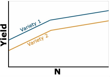
Here yield of the two varieties reacts similarly to N-rate. Thus, there is no interaction between N and variety (Fig. 1). Notice that the lines are parallel, so the effect of the variety is constant as N rate increases. Variety 1 is uniformly superior at each N level and higher levels of N result in improved yield of each variety.
Example 2: Positive Interaction
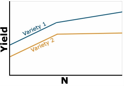
Yield of the two varieties differs based on level of N applied, but the variety 1 always yields better than variety 2 (Fig. 2). The response of each variety depends on the level of N applied. It is no longer constant as in the previous example. The type of interaction is sometimes referred to as a change in the magnitude of the response interaction. Variety 1 is still the highest yielding variety, but the magnitude of its response to N depends on the amount of N applied. With this type of interaction, you can’t evaluate the effect of N independent of variety because the response is different depending on which variety you are talking about. Whenever an interaction tests as significant in the ANOVA, it is important to ignore the main factor means and focus on the interaction means.
Example 3: Negative Interaction
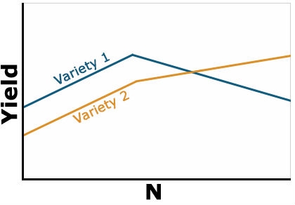
The last type of interaction occurs when the yield response is completely opposite based on the level of N (Fig. 3). Note that the lines in the figure now cross each other. This changes the interpretation drastically because the best variety to grow now depends on the level of N that is applied. You would need to fertilize each variety differently based on the response. This is often called a crossover interaction and it is very important to pay attention when they occur because your recommendation about one factor depends heavily on the level of the other. Often when a crossover interaction occurs one or both main factors involved in the interaction tests as nonsignificant in the ANOVA. When this occurs, you should look at the results very carefully because failure to assess the interaction carefully can result in poor recommendations.
Linear Additive Model for Two-Factor ANOVA
The linear model for a factorial is a simple extension of the linear model. The addition of factors and their possible interaction produce further complexity in the ANOVA. But the effects can be added just as the previous effects were to the linear model.
The linear model for a two-factor ANOVA is:
[latex]Y_{ijk}=\mu+A_i+\beta_j+A\beta_{ij}+\epsilon_{(ij)k}[/latex]
[latex]\text{Equation 1}[/latex]
where:
[latex]Y_{ijk}[/latex] = response observed for the [latex]ijk^{th}[/latex] experimental unit,
[latex]\mu[/latex] = overall mean,
[latex]A_i[/latex] = effect of the [latex]i^{th}[/latex] level of factor A,
[latex]\beta_j[/latex] = effect of the [latex]j^{th}[/latex] level of factor B,
[latex]A\beta_{ij}[/latex] = effect of the interaction between the [latex]i^{th}[/latex] level of factor A and the [latex]j^{th}[/latex] level of factor B,
[latex]\epsilon_{(ij)k}[/latex] = effect associated with the [latex]ijk^{th}[/latex] experimental unit; commonly referred to as error.
True Sources of Variation
Notice that the only change in the linear model from equation 8 is that the treatment structure is modified. We now have sources for factor A, factor B and their interaction. The error structure is not changed; we still have only a single random error for the experiment. Factorial refers to the treatment structure, not the assignment of treatments to experimental units.
For the corn population x hybrid experiment we can rewrite the model to indicate the true sources of variation as:
[latex]\text{Yield}_{ijk}=\mu+POP_i+HYBRID_j+PH_{ij}+PLOT_{(ij)k}[/latex]
[latex]\text{Equation 2}[/latex]
where:
[latex]\text{Yield}_{ijk}[/latex] = corn yield observed for the [latex]ijk^{th}[/latex] plot,
[latex]\mu[/latex] = average yield for the experiment,
[latex]POP_i[/latex] = effect of the [latex]i^{th}[/latex] plant population,
[latex]HYBRID_j[/latex] = effect of the [latex]j^{th}[/latex] hybrid,
[latex]PH_{ij}[/latex] = effect of the interaction between the [latex]i^{th}[/latex] population and the [latex]j^{th}[/latex] hybrid,
[latex]PLOT_{(ij)k}[/latex] = random error effect of the [latex]ijk^{th}[/latex] plot.
Try: Running an ANOVA for a Two-factor CRD in the next screens
Ex. 1: Running an ANOVA for a Two-Factor CRD
R Code Functions
- setwd()
- aov()
- summary()
- <-
- attach()
- subset()
- read.csv()
- detach()
- pf()
- head()
- as.factor()
- interaction.plot()
- as.data.frame()
- aov()
The Scenario
You are an employee for a maize development company in charge of developing new high-yielding maize hybrids for use in central Iowa. For the past 2 years you have been developing A-lines and now you want to test their general combining ability with the company’s elite R-line. Unfortunately, (because it’s Iowa), your plots are savaged by a tornado and bowling ball-sized hail and only 2 of your candidate inbreds remain. You cross these ridiculously fortunate inbreds to the R-line to produce seed for 2 hybrids which are planted the following spring in 3 locations across central Iowa utilizing a randomized complete design with 3 reps at each location. You also plant a standard maize hybrid along with the two you developed to serve as a check within your field (the check is Hybrid C). With the help of your intern, you harvest each plot and calculate the projected bushels/acre.
Source data: The yield data from the hybrids can be found in the file ANOVA 2factorCRD [XLSX]
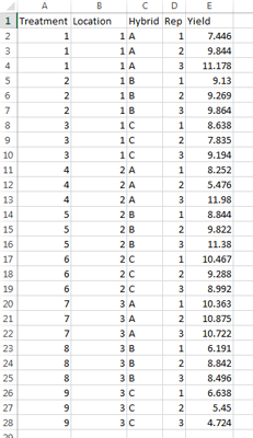
Ex. 1: Data Set
In this data set, you can see that we have columns for treatment, location, hybrid, replication, and the yield in t/ha (Fig. 4). It’s good to remember that while you have 3 hybrids and 3 locations, your total number of treatments is 9, not just the 3 hybrids or the 3 locations. In this activity you will learn how to run a 2-factor ANOVA that will help you choose which of the 3 hybrids you will select and move on to the next stage of testing in your program.
Activity Objectives
- Build and run an ANOVA for a 2 factor model that accounts for population, hybrid, and the interaction between population and hybrid
- Assess whether each individual hybrid is significantly affected by location
Ex. 1: Run the ANOVA
First you need to read in the data set.
Ex9.1<-read.csv(“ANOVA 2factorCRD.csv”, header=T)
head(Ex9.1)
Treatment Location Hybrid Rep Yield
1 1 1 A 1 7.446
2 1 1 A 2 9.844
3 1 1 A 3 11.178
4 2 1 B 1 9.130
5 2 1 B 2 9.269
6 2 1 B 3 9.864
This may not be necessary, but you can use this line of code to make sure that your data is read as a data frame.
Ex9.1<-as.data.frame(Ex9.1)
Ex. 1: Make Adjustments
Check the structure of the data frame; notice that ‘Location’ is considered to be an integer because it’s listed as numbers in the .csv file.
str(Ex9.1)
‘data.frame:27 obs. of 5 variables:
$ Treatment: int 1 1 1 2 2 2 3 3 3 4 …
$ Location : int 1 1 1 1 1 1 1 1 1 2 …
$ Hybrid : Factor w/ 3 levels “A”,”B”,”C”: 1 1 1 2 2 2 3 3 3 1 …
$ Rep : int 1 2 3 1 2 3 1 2 3 1 …
$ Yield : num 7.45 9.84 11.18 9.13 9.27…
You will need to change the ‘Location’ to a factor in order for the analysis to work.
Ex9.1$Location<-as.factor(Ex9.1$Location)
Location<-as.factor(Ex9.1$Location)
Check the structure again and observe that ‘Location’ is now considered to be a factor.
attach(Ex9.1)
Ex. 1: Two-Way ANOVA
Run the ANOVA using the aov() function, just like with one-way designs. The only difference is that now we want to include both factors and their interaction in our model. There are two equivalent ways to do this. The first way explicitly specifies each term; the second way is a shortcut.
str(Ex9.1)
‘data.frame’: 27 obs. of 5 variables:
$ Treatment: int 1 1 1 2 2 2 3 3 3 4 …
$ Location : int 1 1 1 1 1 1 1 1 1 2 …
$ Hybrid : Factor w/ 3 levels “A”,”B”,”C”: 1 1 1 2 2 2 3 3 3 1 …
$ Rep : int 1 2 3 1 2 3 1 2 3 1 …
$ Yield : num 7.45 9.84 11.18 9.13 9.27 …
Or:
Ex9.1.outB = aov(Yield ~ Location*Hybrid, data = Ex9.1)
summary(Ex9.1.outB)
Df Sum Sq Mean Sq F value Pr(>F)
Location 2 9.45 4.726 2.109 0.1504
Hybrid 2 13.09 6.544 2.920 0.0797 .
Location:Hybrid 4 30.25 7.562 3.374 0.0316 *
Residuals 18 40.34 2.241
—
Signif. codes: 0 ‘***’ 0.001 ‘**’ 0.01 ‘*’ 0.05 ‘.’ 0.1 ‘ ‘ 1
Ex. 1: Run Individual ANOVAs
The significant interaction between Population and Hybrid type indicates the simple effects of one factor differ among levels of another factor. One research questions for this example might ask if the yields of each Hybrid type are the same across three Locations. To test the simple main effect of each Hybrid, across three levels of Location, we can perform the analysis as follows:
- Separate the data into subsets, based on Hybrid type
- Run an ANOVA testing the effect of Location in each subset
A = subset(Ex9.1, Hybrid == “A”)
B = subset(Ex9.1, Hybrid == “B”)
C = subset(Ex9.1, Hybrid == “C”)
A.out = summary(aov(Yield ~ Location, A))
A.out
Df Sum Sq Mean Sq F value Pr(>F)
Location 2 6.544 3.272 0.687 0.539
Residuals 6 28.593 4.765
B.out = summary(aov(Yield ~ Location, B))
B.out
Df Sum Sq Mean Sq F value Pr(>F)
Location 2 7.562 3.781 2.935 0.129
Residuals 6 7.729 1.288
C.out = summary(aov(Yield ~ Location, C))
C.out
Df Sum Sq Mean Sq F value Pr(>F)
Location 2 25.594 12.80 19.11 0.0025 **
Residuals 6 4.019 0.67
—
Signif. codes: 0 ‘***’ 0.001 ‘**’ 0.01 ‘*’ 0.05 ‘.’ 0.1 ‘ ’ 1
Ex. 1: Simple Main Effects
Stop and think! Look at the MSE in these simple main effect ANOVAs. They are pretty different. Also, compare dfresidual to the full model ANOVA. The dfresidual (6) are lower in the simple main effect ANOVAs. Since we are comfortable that homogeneity of variance is a reasonable assumption for our data, it is probably safe to use the pooled error for these tests. We can do some calculations to use the pooled error from the overall ANOVA, and its larger number of df (18).
Use pooled error to calculate F and P values for the simple main effects of Location at Hybrid A, B, and C:
Fhybrid.A <- 3.272/2.241
Fhybrid.A
[1] 1.460062
pf(Fhybrid.A, 2, 18, lower.tail – F)
[1] 0.2584485
Fhybrid.B <- 3.272/2.241
Fhybrid.B
[1] 1.687193
pf(Fhybrid.B, 2, 18, lower.tail – F)
[1] 0.2130147
Fhybrid.C <- 12.80/2.241
Fhybrid.C
[1] 0.2130147
pf(Fhybrid.C, 2, 18, lower.tail – F)
[1] 0.2130147
Notice that the P value (0.012) of the test for Hybrid C is less than 0.05, so we would conclude that the yield of this type of Hybrid is affected by Location. The F tests of the Hybrid A and B are not significant at P = 0.05, so we conclude that the yields of these two Hybrids are not influenced by Location.
Ex. 1: Plot the Interaction
attach(Ex9.1)
interaction.plot(Location, Hybrid, Yield, col = c(“green”, “red”, “blue”), main=”Interaction plot of Hybrids A, B, and C”)
The attach() function can be used to make objects within data frames accessible in R with fewer keystrokes. The interaction plot shows that the mean response to Location depends upon the level of Hybrid. Also, we know from our previous tests that Location doesn’t affect the yields of Hybrid A and B, but it has an impact on yield of Hybrid C.
Ex. 1: Interaction Plot
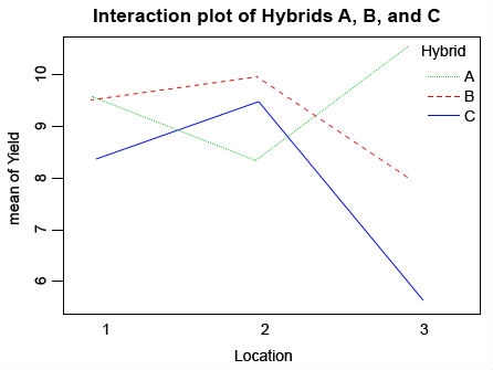
Looking at this interaction plot, you can see that the rank of each line changes depending on the location (Fig. 5). This indicates that there is an interaction between location and environment, but is this interaction significant? Go back to the first ANOVA that you ran and check to see if the interaction is significant, and in this case it is. Based on this information you have gathered from the ANOVAs and your interaction plot, which hybrid would you advance to further testing? Would you choose any hybrid at all? What else do you need to know in order to make this decision?
Ex. 1: ANOVA for 10 Hybrids
Now imagine that the following winter you find some residual seed and replant the inbred lines that were destroyed in the tornado. This time the weather is more cooperative and the following summer you are able to test 10 hybrids at 10 locations (hybrid 10 is the check this time). Use the file “9.1 larger data set” and run the same code as before for the full ANOVA and the interaction plot.
set2<-read.csv(”lesson 9.1 larger set.csv”, header=T)
attach(set2)
set2$Location<-as.factor(set2$Location)
Location<-as.factor(set2$Location)
set2$Hybrid<-as.factor(set2$Hybrid)
Hybrid<-as.factor(set2$Hybrid)
detach(set2)
attach(set2)
str(set2)
‘data.frame’: 300 obs. of 8 variables:
$ Hybrid : Factor w/ 10 levels “1”,”2”,”3”,”4”,..: 1 1 1 1 1 1 1 1 1 1 …
$ Location : Factor w/ 10 levels “1”,”2”,”3”,”4”,..: 1 1 1 2 2 2 3 3 3 4 …
$ Rep : int 1 2 3 1 2 3 1 2 3 1 …
$ overall.Mean: int 170 170 170 170 170 170 170 170 170 170 …
$ G : int 6 6 6 6 6 6 6 6 6 6 …
$ E : num 3.2 11.84 8.05 -1.97 7.41 …
$ error : num -0.209 -0.941 8.491 1.868 0.953 …
$ Yield : num 179 187 193 176 184 …
set2out <- aov(Yield ~ Location+Hybrid+Location:Hybrid, data = set2)
summary(Ex9.1.outA)
Df Sum Sq Mean Sq F value Pr(>F)
Location 9 822 91.3 1.430 0.177
Hybrid 9 18671
Location:Hybrid
Residuals
—
Signif. codes: 0 ‘***’ 0.001 ‘**’ 0.01 ‘*’ 0.05 ‘.’ 0.1 ‘ ’ 1
interaction.plot(Location, Hybrid, Yield, col = c(”green”, “red”, “blue”, “orange”, “black”), main=”Interaction plot of Hybrids 1-10”)
Ex. 1: Interaction Plot of 10 Hybrids
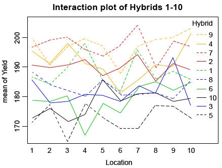
Looking at the plot, you can see that many of the hybrids change rank in different locations (Fig. 6), but if you look at the ANOVA you can see that despite this the interaction is not significant. In real life, you will likely have even larger data sets with many individuals in which case the interaction plot will look very messy and even more difficult to read. This is why it is important to always check the ANOVA and not just rely on the plot.
Ex. 1: Review Questions
- What information can you get from an ANOVA?
- How can you use the ANOVA to make selection decisions?
- What is an interaction?
| Term | Definition |
|---|---|
| setwd(“”) | Set the working directory. Make sure to use the file path where you downloaded your data sets, and not the example I have included! |
| <- | Assignment Operator. Assign value to a variable. Ex: X<-1 means “X gets t”. An = sign does the same thing. |
| read.csv(“”) | Read in a .csv file. Make sure your file name ends in .csv and if you have column names, you need to specify that header=T |
| head(mydataframe) | Returns the top part of the data set specified in the () |
| as.data.frame(mydataframe) | Changes the format of an R object (i.e., a data set) to a data frame. This is one of the more common formats for working with a data set. |
| str(mydataframe) | Returns the structure of an R object |
| attach(mydataframe) | Attach an R object so that R knows this is what you want to work with at this moment. |
| detach(mydataframe) | Detaches the R object you were working with |
| as.factor(mydataframe$variance) | Changes a variable within an R object to a factor variable. An example is when you have variables designated with numbers but they are meant to be categorical variables so you use this function to tell R that. |
| aov(y ~ A + B + A:B, data=mydataframe) | Perform a 2-factor analysis of variance on an R object. |
| summary() | Returns the summary of an analysis. |
| subset(mydataframe, variable == “variable value”) | Subsets a variable within a data frame based on a particular variable value. |
| pd(F-value, df1, df2, lower.trial = F) | Calculate the P-value. Lower.tail=F means P[X > x] |
| interaction.plot(x.factor, trace.factor, response,…) | Create interaction plot. X.factor is the factor that forms the x-axis, trace.factor is another factor whose levels for the traces, response is the numeric variable giving the response. You can also add specific colors to the plot with col=c”color1″, “color2” and a title with main = “title” |
ANOVA and Experimental Design
Experimental Design and Analysis
You will recall from Chapter 1 on Basic Principles that experimental design refers to the manner in which treatments are assigned to experimental units (plots). In this chapter, we have assumed that all treatments are applied at random to the entire set of experimental units used in the experiment. This is what is known as a Completely Random Design (CRD). In a CRD every experimental unit has the same chance of receiving any given treatment.
Experimental design allows researchers to control factors influencing outcomes.
Statistical analysis is a powerful approach to understanding collections of data. The analysis employed depends on the type of data and the manner in which it was collected. There are two broad categories or approaches to research that commonly are used: observational experiments and designed experiments.
Observational experiments involve collecting data from a population of individuals to which no treatments have been applied. They are descriptive in nature and usually involve studying the relationships among two or more variables of interest. It is important to understand that the variables studied in an observational experiment occur naturally and are not manipulated by the researcher in any way. An example of an observational experiment would be a comparison of groundwater nitrate concentrations among several Iowa counties.
Designed experdesigned experimentsiments differ from observational experiments in that data are collected from units that have been manipulated by the researcher in some way before the data are collected. This is often described as applying treatments to experimental units. Some good agricultural examples of treatments are the application of specific fertilizer rates and the planting of specific crop varieties for the purposes of comparison. In agronomic terms, the smallest entity to which treatments are applied is usually a field plot.
Characteristics of designed experiments:
- Replication – treatments are repeated two or more times on different experimental units (plots)
- Randomization – treatments are randomly assigned to experimental units (plots)
- Design Control – how treatments are applied to various groupings and sizes of experimental units (subplots, plots, blocks, locations)
We use a CRD when we expect the magnitude of the plot effect to be similar among all the plots used in the experiment. Statisticians refer to this condition as homogeneity, and it is assumed when we use a CRD. The CRD is a common design (Fig. 7); there are many cases where its use is appropriate. For example, in a growth chamber, we might have 25 flats filled with sand, each planted with 30 wheat seeds, 5 reps of each of 5 varieties.
However, whenever there are not enough plots with similar characteristics to accommodate all the treatments and replications in an experiment, alternative designs should be considered to improve the precision of the experiment. We will learn more about this as we study other designs in subsequent chapters.
Randomly Assign Treatments
There are many ways to randomly assign treatments to experimental units. The use of a table of random numbers is described in the text. This method involves listing all the treatments and their replications and assigning a random number from a table of random numbers to each one. This random order is then matched to a predetermined order of experimental units. A far easier approach is to use a computer to randomize treatments. You can use Excel or R to randomize an experiment.
Ex. 2: Randomized Complete Design using R
R Code Functions
- setwd()
- paste()
- sample()
- <-
- data.frame()
- write.csv()
- read.csv()
- write.table()
- as.data.frame()
- head()
- matrix()
The Scenario
You are an employee for WinField Solutions interested in studying the impact of Japanese beetles (Popillia japonica) on soybeans and recently two new insecticides have come on the market. To test their effectiveness against Japanese beetles, you choose to test the insecticides on the three most commonly grown cultivars in Iowa. You want to design an experiment where each insecticide is paired with each cultivar and replicated four times. To account for differences within your field you want to test these pairs in a completely randomized design. Ultimately you wish to be able to show clients which insecticide/cultivar pairs are the most effective at preventing damage from Japanese beetles.
Ex. 2: Activity Objectives
- Randomize a list of all the insecticide/cultivar pairs.
- Assemble the list into a rectangular field plot.
Start by setting the working directory. As always, you need to use your own chosen directory, this is just an example.
setwd(“C:/Users/UserName/Desktop/SAS to R”)
After you read in the data, be sure to check the head to make sure it was read in properly.
crd<-read.csv(“Randomization 2factor CRD.csv”, header=T)
head(crd)
Insecticide Cultivar
1 1 1
2 2 1
3 1 2
4 2 2
5 1 3
6 2 3
Ex. 2: Randomize as Pairs
Because we have two types of treatments and we want them to be randomized as pairs, it makes sense to have insecticide and cultivar treatments be represented as a single value such as ‘1–2’ to represent insecticide 1 and cultivar 2. It will be up to you to decide which insecticide and cultivar will be represented by each number. To do this in R, we can merge the two columns and separate them with ‘–‘ with this code:
IC <- as.factor(paste(crd$Insecticide, crd$Cultivar, sep = “–”))
IC
[1] 1–1 2–1 1–2 2–2 1–3 2–3 1–1 2–1 1–2 2–2 1–3 2–3 1–1 2–1 1–2 2–2 1–3 2–3 1–1 2–1 1–2 2–2
[23] 1–3 2–3
Levels: 1–1 1–2 1–3 2–1 2–2 2–3
Originally, I used just one ‘-‘ between the numbers but I found that when I imported this into Excel, it is read as a date and it is not easy to get Excel to display them properly. Now that we have made a vector of the treatment combinations, we need to create another vector of numbers that will list the order of the plots, so we need the list to be the same length as the total number of plots (24). This is important for when we randomize the order.
v<-1:24
v
[1] 1 2 3 4 5 6 7 8 9 10 11 12 13 14 15 16 17 18 19 20 21 22 23 24
Now we combine the treatments with the vector we just created.
data <- data.frame(Treatment=IC, tempplot=v)
data
Treatment tempplot
1 1–1 1
2 2–1 2
3 1–2 3
4 2–2 4
5 1–3 5
6 2–3 6
7 1–1 7
8 2–1 8
9 1–2 9
10 2–2 10
11 1–3 11
12 2–3 12
13 1–1 13
14 2–1 14
15 1–2 15
16 2–2 16
17 1–3 17
18 2–3 18
19 1–1 19
20 2–1 20
21 1–2 21
22 2–2 22
23 1–3 23
24 2–3 24
Ex. 2: Randomize the Order
Now that we have created the data set that we can work with, we can randomize the order of the treatments.
randdata <- data[sample(1:nrow(data)),]
randdata
Treatment tempplot
13 1–1 13
22 2–2 22
4 2–2 4
23 1–3 23
2 2–1 2
24 2–3 24
12 2–3 12
17 1–3 17
9 1–2 9
7 1–1 7
18 2–3 18
8 2–1 8
19 1–1 19
21 1–2 21
11 1–3 11
3 1–2 3
20 2–1 20
5 1–3 5
15 1–2 15
6 2–3 6
1 1–1 1
10 2–2 10
16 2–2 16
14 2–1 14
Now if you look at the order of the treatments, you can see that they have been completely randomized. However, because the list of 1-24 is also out of order, this can be a little confusing if you are trying to get a planting plan together. We can keep the treatments randomized but we can have the plot numbers be in order with this code:
treatment<-as.factor(randdata$Treatment)
treatment
[1] 1–1 2–2 2–2 1–3 2–1 2–3 2–3 1–3 1–2 1–1 2–3 2–1 1–1 1–2 1–3 1–2
[17] 2–1 1–3 1–2 2–3 1–1 2–2 2–2 2–1
Levels: 1–1 1–2 1–3 2–1 2–2 2–3
treatment<-as.factor(randdata$Treatment)
finaldata
Treatment tempplot
1 1–1 1
2 2–2 2
3 2–2 3
4 1–3 4
5 2–1 5
6 2–3 6
7 2–3 7
8 1–3 8
9 1–2 9
10 1–1 10
11 2–3 11
12 2–1 12
13 1–1 13
14 1–2 14
15 1–3 15
16 1–2 16
17 2–1 17
18 1–3 18
19 1–2 19
20 2–3 20
21 1–1 21
22 2–2 22
23 2–2 23
24 2–1 24
Ex. 2: Matrix Form
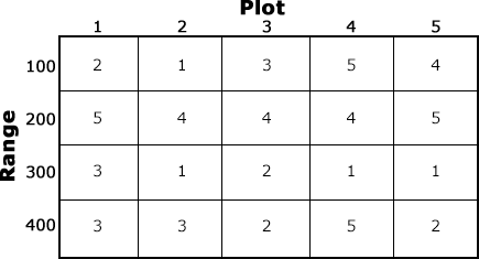
Finally, if you know you want to plant these soybean plants in a rectangular field, you can use this code to convert your randomized treatments to a matrix form.
A = matrix((treatment), nrow=4, ncol=6)
A
[,1] [,2] [,3] [,4] [,5] [,6]
[1,] “1–1” “2–1” “1–2” “1–1” “2–1” “1–1”
[2,] “2–2” “2–3” “1–1” “1–2” “1–3” “2–2”
[3,] “2–2” “2–3” “2–3” “1–3” “1–2” “2–2”
[4,] “1–3” “1–3” “2–1” “1–2” “2–3” “2–1”
Remember, this is a completely randomized design, not a randomized complete block design. You may well have a field design where you have a section of the same cultivar or insecticide repeated several times, but it will still be random.
You can export your randomized list and field layout as a text file or .csv file.
write.table(finaldata, file = “Randomized list.txt”)
write.table(A, file = “field layout.txt”)
write.csv(finaldata, file = “Randomized list.csv”)
write.csv(A, file = “field layout.csv”)
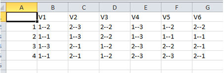
Ex. 2: Visualizing Results in Excel
This way you can save your results and you can do further visualization in programs like Excel.
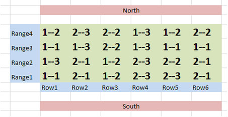
For example (Fig. 8):
You can start with this and add ranges and row labels to get a clearer idea of what the field layout will be like Fig. 9.
Ex. 2: R Code Glossary
| Term | Definition |
|---|---|
| setwd(“”) | Set the working directory. Make sure to use the file path where you downloaded your data sets, and not the example I have included! |
| <- | Assignment Operator. Assign value to a variable. Ex: X<-1means “X gets 1”. An = sign does the same thing. |
| read.csv(“”) | Read in a .csv file. Make sure your file name ends in .csv and if you have a column names, you need to specify that header=T. |
| head(mydataframe) | Returns the top part of the data set specified in the (). |
| as.factor(mydataframes$variable) | Changes a variable within an R object to a factor variable. An example is when you have variables designated with numbers but they are meant to be categorical variables so you use this function to tell R that. |
| paste(…,sep=””) | Concatenate strings after using sep string to seperate them. paste(“x”,1:3,sep=””) returns c(“x1″,”x2″,”x3”) paste(“x”,1:3,sep=”M”) returns c(“xM1″,”xM2″,”xM3”) paste(“Today is”, date()) |
| data.frame() | Combines variables into a single data frame. |
| sample() | Returns a random permutation of a vector. |
| Matrix((variable), number of rows=, number of columns) | Takes a vector and transforms it into a matrix with the specified dimensions of rows and columns. You need row and column numbers that multiply to be the total number of individuals, or you will get an error. |
| write.csv(mydataframe, “.csv”) | Write your data frame to a .csv file. |
| write.table(mydataframe, “.txt”) | Write your data frame to a .txt file. |
Error Structure
Once the randomization is completed and the experiment properly conducted according to plan, the error structure for the experiment is, at least partially, determined. For the CRD, for example, we do not have a blocking factor because treatments are assigned to experimental units completely at random. In chapter 11 on Randomized Complete Block Design, we will introduce another type of design, the Randomized (Complete) Block Design, or RCBD, in which some restrictions are put on the randomization. For the RCBD, there is yet another recognizable source of variation in the ANOVA, that for blocks, as you will see in chapter 11.
Summary
Factorial Experiments
- Involve more than one treatment factor.
- Allow exploration of combinations of factors, interaction
- Refers to the treatment structure, not how treatments are assigned to plots.
Interaction
- Differential response of one factor at different levels of another.
Linear Model
- Factorial Linear Model is simple extension for more detail on treatment factors and interaction.
Experimental Design
- Determines model and ANOVA.
- CRD has treatments assigned to experimental units completely at random.
How to cite this chapter: Mowers, R., M., L. Harbur, K. Moore, L. Merrick, A. A. Mahama, & W. Suza. 2023. Two Factor ANOVAs. In W. P. Suza, & K. R. Lamkey (Eds.), Quantitative Methods. Iowa State University Digital Press.
A design where every plot has an equal chance of any treatment.
An experiment in which variables studied occur naturally and are not manipulated by the researcher.
An experiment in which variables studied have been intentionally manipulated by the researcher.
A procedure or manipulation for which you wish to measure a response. Some good agronomic examples are the application of specific fertilizer rates and the planting of specific crop varieties for the purposes of comparison.
The smallest entity to which treatments are applied.
An aspect of experimental design in which the treatment array is duplicated several times.
Process of assigning experimental units without any bias. Usually executed by random number generation.
Application of restrictions on randomization in the design of an experiment for the purpose of better controlling recognizable sources of variation; for example, blocking to control soil variation in a randomized complete block experiment.
A population is considered to be homogeneous when all members have similar traits.
