
Chapter 11: Randomized Complete Block Design
M. L. Harbur; Ken Moore; Ron Mowers; Laura Merrick; Anthony Assibi Mahama; and Walter Suza
It is important when conducting an experiment that the experimental units be as homogenous as possible. This ideal may be met without much difficulty in a lab or within a field with particularly uniform soils. In many field locations, however, the landscape can vary greatly over a short distance. How can we assure, then, that an observed agronomic difference is the result of a specific treatment, rather than the result of the experimental units to which it was allocated? In other words, how do we prevent our treatment results from being confounded with our experimental units? The Randomized Complete Block Design (RCBD) offers one solution.
- How heterogeneity of experimental units can reduce the sensitivity of an experiment
- How the Randomized Complete Block Design (RCBD) can be used to reduce the heterogeneity of experimental units
- How to conduct the analysis of variance (ANOVA) for an experiment that employs the RCBD
- How to test for the efficiency of the RCBD versus that of the Completely Randomized Design
Blocking
The rationale for blocking is to achieve homogeneous experimental units within blocks. In Chapter 1 on Basic Principles, you learned about the importance of replication in designing a valid experiment. We applied those concepts in Chapter 8 on The Analysis of Variance (ANOVA) when we introduced the analysis of variance. Treatments and replications were assigned to experimental units through the process of randomization. The result of this effort is referred to as a Completely Random Design (CRD).
The CRD is an appropriate experimental design when all experimental units are assumed to be similar or homogeneous (as statisticians like to say). If this is the case, then any observed differences among treatments will cause us to conclude that there was a treatment effect. As mentioned in the introduction, however, homogeneity of experimental units can be difficult to achieve in field plot experiments.
Heterogeneity
Heterogeneity of experimental units presents two problems. First, the failure to recognize differences between experimental units may lead us to conclude that differences in our variates are the result of the treatments applied, when they were actually caused by the pre-existing condition of the experimental units.
Variance of the Error
Differences between plots (experimental units) not related to the treatments applied to them can inflate the variance of the error associated with the experiment. Recall from Chapter 8 on The Analysis of Variance (ANOVA) that we tested the significance of our treatment using an F-test (Equation 1 below).
If the residual mean square error is increased, then the treatment mean square must also increase in order to maintain the same F-value. In other words, the greater the pre-existing differences between our plots (experimental units), the greater and more profound the difference between treatments must be just to be recognized as statistically significant. Heterogeneity of experimental units thus reduces the sensitivity of our experiment.
[latex]\small F = \dfrac{TMS}{RMS}[/latex]
[latex]\textrm{Equation 1}[/latex] Formula for calculating F value.
where:
[latex]\small TMS[/latex]= treatment mean square,
[latex]\small RMS[/latex]= residual (error) mean square.
How to Block
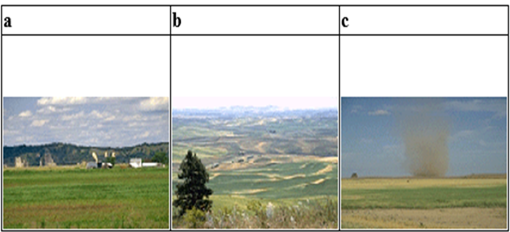
The first step in using the RCBD is to recognize the source(s) of potential heterogeneity among plots (experimental units). In field research, this potential most often exists between plots situated on different soil map units, for example, as the slope changes. We viewed some of the potential differences in soils related to landscape in Study Question 1. There are many other possible sources of heterogeneity among plots, though. These map units often differ in their yield potential, with the result that some of the variation in the yield measurement is due to the plot location. One example of site heterogeneity is found in Fig. 2.
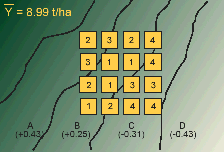
In the map in Figure 1, we have four map units (A-D) labeled with the difference in yield between each map unit and the mean for the entire field. As we move from map unit A across to map unit D, the yield potential decreases. In such a case, we say that we have a “production gradient” across the map units. Now let’s suppose that we are comparing four different levels of fertilizer (0, 50, 100, 150 kg/ha). If we used a completely randomized design (CRD) across these map units, we risk the possibility of placing all of the high-fertility treatments on extreme map units. This would lead to an unfair comparison of the treatments.
Answer the following question using the treatment map above.
Treatments
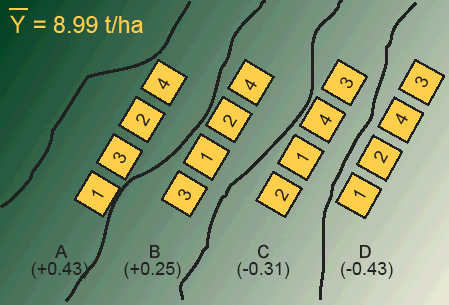
In blocking, we generally place an equal-sized block on every map unit. Each block, in this case, contains four experimental units (plots). Each treatment is applied to one experimental unit within the block (Fig. 3).
Each block can be thought of as a replication. Every treatment is forced to occur within each block. Treatments are randomly allocated within each block so that separate randomization is made for each block. In this way, the treatments are prevented from being affected by a second, unrecognized source of heterogeneity that could exist between experimental units within the blocks.
Design Control
Forcing each treatment to occur once in every block is sometimes referred to as a restriction on randomization. The restriction in the case of a RCBD is that every treatment must occur in every block. In a CRD, every plot would have the same chance of receiving any treatment, so there is no restriction on randomization; hence the name.
Blocking is a form of design control that was discussed in Chapter 1 on Basic Principles. It is one of the three characteristics of designed experiments (do you remember the other two?). Blocking in a field experiment amounts to grouping plots into more similar sets such that the variation associated with the blocks (whatever is causing them to differ) can be estimated and associated with the block. In a CRD, this variation would be associated with and show up in the Error MS, thus inflating the estimate and reducing the precision of the experiment. When blocking is effective (i.e. there is some variation in the measured response associated with the blocking criterion), this variation is removed from the Error MS and the ability to detect true treatment differences (i.e. precision of the experiment) is improved.
Further Thought: Discussion
What other possible influences could affect each block beyond the known yield potential gradient?
Randomization
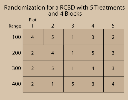
Fig. 4 below illustrates a RCBD randomization scheme. Notice that the Blocks are numbered 100, 200, 300, and 400 and that each of the 5 treatments is on one plot in each block.
Randomization should be done using some sort of randomization method, not just arbitrarily. This precludes any bias which may be unintentionally introduced due to the assignment of treatment. Check out the exercise in the next screens to learn how to randomize treatments for a RCBD using Excel.
Ex. 1: Randomizing Treatments for a RCBD
As we said before, experimental design is really about how treatments are assigned to experimental units (plots). In the case of the randomized complete block design (RCBD), treatments are blocked into groups of experimental units that are similar for some characteristic. In field experiments, treatments are usually blocked perpendicular to some perceived gradient present in the field. The gradient may be related to such characteristics as soil properties, previous crop history, or any number of other factors that can occur naturally or unnaturally in a field. In a RCBD, treatments are allotted to plots at random within each block of experimental units (plots) such that within any given block, each plot has the same probability of receiving a particular treatment as any other. The only restriction is that every treatment has to occur in every block.
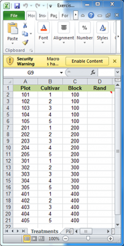
For the purpose of this exercise, we will develop a plot plan for an oat variety trial experiment. The treatments consist of five cultivars replicated four times for a total of twenty plots. The treatments and plots are listed in the Treatments worksheet of the Excel file QM-mod11-ex1data.xls. A map of the field layout is presented in the Plot Plan worksheet. Our goal is to randomize the plot order within blocks and permanently associate it with the treatments.
Ex. 1: Create a Random Assignment
Randomly assign the five oat cultivars to each of the four blocks identified in the Treatments worksheet. The idea now is to create a random order of the treatments under the restriction that each Cultivar must occur once in each Block.
Steps:
- Enter the formula =RAND() in cell D2.
- Copy the formula in cell D2 to cells D3:D21. A fast way to do this is to double-click the square that appears in the lower right-hand corner of the cell when you select cell D2. The RAND() function will return a random number between 0 and 1 to each cell the formula is copied to.
- Using your mouse, select all the cells in the Cultivar, Block, and Rand columns, including the column headings (B1:D21). Do not select the Plot column!
- Select Sort from the Data menu at the top of the main window.
- In the Sort by box in the Sort dialog box, select Block.
- If not already present, add another sort level by clicking on Add Level.
- In the second Sort by box, select Rand and then click OK.
Ex. 1: Finished Random Assignment
You should now have a random assignment of Cultivars in column B, and each cultivar should occur once in every block. Your worksheet should look something like Fig. 5.
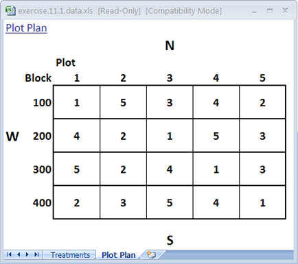
Ex. 1: Plot Plan
The treatments are now sorted according to plot order. Look at the Plot Plan worksheet to see the field layout of the plots according to the new randomization (Fig. 6). Your plan should look something like the one below. Note that every cultivar occurs once in every block. However, the order of treatments within each block will vary with each randomization.
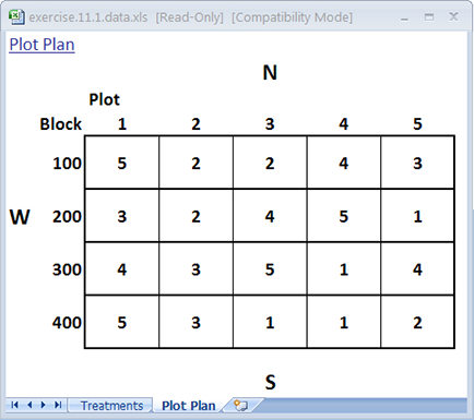
Ex. 1: RCBD vs. CRD Randomization
You may have noticed that randomizing treatments for the CRD and RCBD follow a similar process in Excel. The main difference is in the number of sort levels you use. In the CRD, only one sort level was used which corresponded to the random number generated by the RAND() function. In the case of the RCBD, you used two sort levels: 1) the first one assigned to Blocks, and 2) the second assigned to the random number. You can compare and contrast the plot map from the previous page for an RCBD with one generated for a CRD by removing the first sort level so that the only one that remains is the random number.
The restriction on randomization has been removed so that any cultivar can be assigned to any plot (Fig. 7).
Ex. 1: R Code Functions
- matrix
- for
- gl
- runif
- cbind
- _[order]
Experimental design is really about how treatments are assigned to experimental units (or plots). In the case of the randomized complete block design (RCBD), treatments are blocked into groups of experimental units that are similar for some characteristic. In field experiments, treatments are usually blocked perpendicular to some perceived gradient present in the field. The gradient may be related to such characteristics as soil properties, previous crop history, or any number of other factors that can occur naturally or unnaturally in a field. In a RCBD, treatments are allotted to plots at random within each block of experimental units (plots) such that within any given block, each plot has the same probability of receiving a particular treatment (location) as any other. The only restriction is that every treatment has to occur in every block.
Ex. 1: Maize Yield Test
You are a maize breeder in charge of designing a field for a yield test of 3 synthetic maize populations. The field has never been used before by your company, and the area surrounding the field is known to have very localized deposits of clay which inhibit root growth and thus negatively affect the yield of plants planted directly on top of the deposits. You want to account for the heterogeneity of the field by assigning each of the 3 maize populations to one of the 3 positions in each of 3 blocks.
In other words, you want to create a random order of the three populations (or treatments) within each block under the restriction that each population must occur once in each block. To make the coding a bit easier for this exercise, we will rename Population 7.5 to Population 1, Population 10.0 to Population 2, and Population 12.5 to Population 3.
Exercise 1:
We will learn two ways to do this. The first way will take a little longer than the second but involves less coding. The second way will be much faster than the first. However, it will involve at least a basic understanding of some coding tools, such as loops.
Ex. 1: Creating a Field
Let’s start by creating a matrix of all zeros, where each entry represents a plot that will be assigned to a cultivar, and each column represents a block. We have 3 cultivars in each of the 3 blocks, thus the dimensions of this ‘field’ matrix should be 3×3. We will use the matrix command to create the field in R. In the Console window, enter in the parenthesis after matrix, the 0 indicates the type of element we want the matrix to be composed of (i.e., in this case, zeros because we are going to fill in the cultivar numbers, which will be randomly assigned to each plot in each block). The first 3 indicates the number of rows we want in the matrix; since we have 3 populations in each block, we need our matrix to have 3 rows. Finally, the second 3 indicates that we want 3 columns (blocks) in our matrix.
field<-matrix(0,3,3)
Have a look at the field you’ve created. Enter field into the Console.
field
[,1][,2][,3]
[1,] 0 0 0
[2,] 0 0 0
[3,] 0 0 0
Ex. 1: Creating a Vector
Now, let’s create a vector representing the cultivars we have in our breeding program. We’ll accomplish this by using the gl command. This command allows us to create a vector (or column) of factor variables. In the parenthesis after the gl command, the first entry (3) indicates the number of factor levels, and the second number (1) indicates the number of replications of each factor variable. You may be asking yourself why we are not entering a 3 for the number of replications, as we have 3 randomized complete blocks. The reason we do not enter a 3 for replications is due to the fact that we will create randomized complete blocks individually and enter them into each block (column) in the field matrix. This will become apparent in the following steps.
Enter into the Console:
pop<-gl(3,1)
pop
[1] 1 2 3
Levels: 1 2 3
Ex. 1: Vector with 3 Entries
Now let’s create a vector with 3 entries, where each entry is a random number between 0 and 1. We’ll use the runif command to do this. This command is used by entering the number of entries of numbers between 0 and 1 you want your vector to be composed of in parenthesis after the runif command (i.e. for this example, we will enter 3, since we have 3 maize populations). Let us call this vector with 3 entries of random numbers between 0 and 1 rand. Create the vector rand, then look at it by entering the vector name (rand).
rand<-runif(3)
rand
[1] 0.1165839 0.5730972
0.3469669
Ex. 1: New Matrix with Block
Now, let us create a new matrix called block by putting the cultivar and rand vectors together, so each random number in the rand vector corresponds to one of the 3 maize populations. The cbind command can be used to put two vectors together. The command is used by entering the cbind command followed by the two vectors you want to be put together (or concatenated) in parenthesis separated by a comma. Create the matrix called block with the cbind command, then look at the matrix by entering the name of the matrix (block).
block<-cbind(pop,rand)
block
pop rand
[1,] 1 0.1165839
[2,] 2 0.5730972
[3,] 3 0.3469669
Ex. 1: Ordering the Population in Block
We can now order the maize populations in the first column of the block matrix by each of the 3 population’s corresponding random number in the rand vector. We will use the order command to sort the populations based on their corresponding number in the rand column, by the population with the smallest random number first to the population with the largest random number last. The population with the smallest random number is Population 1 (0.1165839), and the population with the largest random number is Population 2 (0.5730972). Thus, the order for this randomized complete block should be 1,3,2. We will now go through the order command.
Let us call this randomized complete block randblock. Create matrix randblock and take a look at it by entering the following in the Console.
block<-cbind(pop,rand)
block
pop rand
[1,] 1 0.1165839
[2,] 2 0.5730972
[3,] 3 0.3469669
Ex. 1: Filling the Block
To use the order command, we first write the matrix or vector that we’d like ordered (i.e., in this case, block), followed by brackets. Then, we write the command order followed by the column that we would like the ordering of the rows based off of (i.e., in this case the second column of the block matrix, which contains the random numbers between 0 and 1 for each population. Note: the row number is left blank in the brackets before the comma block[order(block[,2]),] to specify that we want all of the rows sorted based on the values of column 2 in the block matrix. Since the second column in the block matrix is the random number column, this is the column that we want to order the populations by; thus, we enter block[,2] to specify we want the rows ordered based on the values in the second column in the block matrix. The default of the order function is to sort in a ascending order, with the lowest value at the top of the column and the highest value at the bottom. We must now enter this randomized block into the first block (column) of the field matrix we created previously. We’ll do this by setting the first column of the field matrix (specified by field[,1]) to equal the first column of the randblock matrix (specified by randblock[,1]). Carry out this operation, then look at the field matrix to make sure you’ve entered the first column from the randblock matrix into the field matrix.
field[1,]<-randblock[1,]
field
[,1] [,2] [,3]
[1,] 1 0 0
[2,] 2 0 0
[3,] 3 0 0
Again, we specify the first column of the field matrix with field[,1], and set it equal to the first column of the randblock matrix, specified by randblock[,1]. Note: The order of the cultivars in the first column of your field matrix may not be the same as in this lesson due to the randomization process.
To fill in the rest of the blocks, carry out all of the same steps you just did, but when entering the next block into the field matrix, change the
field[,1]<-randblock[,1] to field[,2]<-randblock[,1]
to specify that you want to enter the randomized order for the second block (or column) in the field matrix.
Ex. 1: Review RCBD Method 1
To summarize what we’ve just learned, the first method for creating 3 randomized complete blocks with 3 populations is reviewed succinctly below.
First, we create a field matrix of all zeros, with the dimensions of the number of entries in each block, and the number of blocks desired (i.e., in this case we have 3 populations or entries, and 3 blocks).
field<-matrix(0,3,3)
Then, go through steps 1-5 (presented below) 3 times. After each time through steps 1-5, add 1 to the column indicated in the field matrix in step 5. For example, the second time through steps 1-5, step 5 will be field[,2]<-randblock[,1], and the third time through step five will be field[,3]<-randblock[,1], etc.
cultivar<-gl(3,1)
rand<-runif(3)
block<-cbind(cultivar,rand)
randblock <- block[order(block[,2]),]
field[,1]<-randblock[,1]
Have a look at the field you’ve just created:
field
[,1] [,2] [,3]
[1,] 1 1 2
[2,] 3 3 1
[3,] 2 2 3
Ex. 1: RCBD Method 2
This method can save time in comparison with the first method, especially if you have many treatments that you want randomized in many blocks. The two methods are computationally equivalent, however the second method utilizes a loop command to repeat the operations that we previously did for each block in Method 1.
We can use a for loop to go through a set of operations a specified number of times. Using the for loop, we must first assign an iteration variable, which corresponds to the number of times the set of operations has been completed. For example, if we assign i=1:3 as the iteration variable, the first time through the set of commands i=1, the second time i=2, the third time i=3. In this example, we’ll use the letter i to indicate the iteration variable in our loop.
Let’s clear the entire data frame before starting Method 2. Use the rm(list=ls()) command to clear the entire data frame/environment. The upper-right window should now be clear of all variables and data.
rm(list=1s())
Ex. 1: Creating a Field Matrix
Great! Now create the field matrix in the same way as in Method 1.
rm(-matrix(0,3,3)
Now we need to enter the loop with the number of cycles, or iterations we want carried out. In this case, we want to create 3 randomized complete blocks, so we the total number of iterations is 3. Enter the for command into the Console with the iteration variable i ndicating that we want 3 iterations carried out
for (i in 1:3)
Good, we have indicated that we want i to be our iteration variable ranging from 1 to 3. Now, we need to enter the bracket { , then enter lines 1-5 from the method 1 code with line 5 ending in a } bracket.
{pop<-gl(3,1)
rand<-runif(3)
block<-cbind(pop,rand)
randblock <- block[order(block[,2]),]
field[,i]<-randblock[,1]}
Ex. 1: Finished Field Matrix
Look at line 5 for Method 2 directly above. Do you notice anything different than line 5 in Method 1? Instead of manually entering the block number in the field[,1]<-randblock[,1] command, we simply enter i, so that line 5 in Method 2 becomes field[,i]<-randblock[,1]. The value of i is 1 for the first iteration, 2 for the second iteration, and 3 for the third iteration. This can save us a lot of time if we are trying to create many randomized complete blocks for many treatments.
Let’s now go through method 2 in its entirety.
for (i in 1:3)
{pop<-gl(3,1)
rand<-runif(3)
block<-cbind(pop,rand)
randblock <-
block[order(block[,2]),]
field[,i]<-randblock[,1]}
Look at the field you’ve just created.
field
[,1] [,2] [,3]
[1,] 1 1 2
[2,] 3 3 1
[3,] 2 2 3
Ex. 1: Review RCBD Method 2
To reiterate, Method 2 is accomplished by first creating the field matrix.
field<-matrix(0,3,3)
Then entering the for command, specifying the iteration variable (i.e., i in 1:3)
for (i in 1:3)
and finally entering a { bracket, lines 1 to 5 from Method 1, with a } after the final line (line 5).
{cultivar<-gl(3,1)
rand<-runif(3)
block<-cbind(cultivar,rand)
randblock <- block[order(block[,2]),]
field[,i]<-randblock[,1]}
Linear Additive Model
The Linear Additive Model also applies for the RCBD. In Chapter 8 on The Analysis of Variance (ANOVA) we introduced the linear additive model in describing the analysis of variance. The model showed how the measured or dependent variable is affected by different factors in the model (independent or classification variables). According to the linear model, the observed result can be estimated by adding (summing) the effects of the model terms. By introducing blocking into the experimental design, another possible source of variation is included in the linear additive mode that is associated with blocks. Thus, the model for a RCBD includes an additional term for blocks. The error term can now be thought of as that variability among plots (experimental units) that cannot be accounted for by blocks or treatments.
The linear additive model for the RCBD must include the effects of blocking, treatment(s), and error (Equation 2). The model for a single-factor RCBD is:
[latex]Y_{ij}=\mu+\beta_i+T_j+\beta{T}_{ij}[/latex]
[latex]\textrm{Equation 2}[/latex] Linear Additive Model.
where:
[latex]Y_{ij}[/latex] = response observed for the [latex]ij^{th}[/latex] experimental unit,
[latex]\mu[/latex] = grand mean,
[latex]B[/latex] = block effect,
[latex]T[/latex] = treatment effect,
[latex]BT[/latex] = block error x treatment interaction.
Differences in Models
This model differs from the linear additive model for the CRD in two ways. First, it differs by including blocks as an effect. Blocks capture the effect related to the blocking criterion, which is often soil heterogeneity in field experiments. The RCBD model, by having a block effect, inherently includes a restriction on randomization. The RCBD is not completely randomized — instead, each level of the treatment is “forced” to occur in each block.
The second difference is that the block x treatment interaction is the error term. Why should we use this interaction to test the effect of treatment? The answer is that we test treatment differences to see if they remain relatively large compared with their random changes for different blocks. These random changes in treatments over blocks comprise the BT interaction.
Suppose that soybean yield means for three herbicide treatments are 2.7 t/ha for herbicide A, 3.0 for B, and 3.3 for C. If these differences remain fairly consistent over each block, the block x treatment interaction will be small relative to the mean yield differences, and the F-ratio of treatment MS to error (BT interaction) will be large. In effect, we are testing whether the yield differences remain relatively large in comparison with their (random) changes over blocks, i.e., block x treatment interaction. The block x treatment is the proper error term for testing for treatment differences and it is used for the F-Test in the ANOVA. A large F-value implies treatment differences are large relative to the error.
Treatment Differences

In both graphs in Fig. 8, the average soybean yields are the same (2.7, 3.0, and 3.3 t/ha). We trust the results more if these differences are consistent across blocks (left-hand side). When the B x T interaction is large, (right-hand side), the random error obscures the treatment differences.
Estimate Effects Using ANOVA
Perhaps the linear model will be clearer if we use an example. Recall the corn population experiment from Chapter 5 on Categorical Data—Multivariate. In that experiment, corn was planted at three populations in order to determine the effect on grain yield. If we treat the repetitions as being blocks, the linear model for that specific experiment is (Equation 3):
[latex]\small Y_{ij}=\mu+Blk_i+POP_j+BlkxPOP_{ij}[/latex]
[latex]\textrm{Equation 3}[/latex] Linear Additive Model.
where:
[latex]\mu[/latex] = grand mean,
[latex]\small Blk[/latex] = block effect,
[latex]\small POP[/latex] = population effect.
The linear model provides a convenient method of listing the effects which are to be estimated using an ANOVA. As you will see, every effect from the linear model (with the exception of the mean) will be included in the ANOVA table. The arguments you list in the aov() function in R correspond directly to the terms that comprise the linear additive model.
R Code Functions
- attach()
- as.factor()
- summary()
- aov()
In this example, you will learn how to analyze data from an experiment that has a restriction on randomization. This exercise will give us an opportunity to evaluate how blocking affects the sum of squares for our model. More specifically, it will allow us to discern how Total SS are partitioned between the two designs (blocking vs. not blocking).
Exercise 2: Analyze an RCBD experiment
We return to the synthetic maize population scenario which we used in the previous exercise, where we created randomized complete blocks. You are again a maize breeder and have now been asked by your supervisor to analyze the yield data for the 3 synthetic maize populations that were planted in a yield trial in 3 randomized complete blocks. Conduct an ANOVA on this data with cultivar and block as factors.
Ex. 2: Beginning Analysis
Reading the DataTo begin the analysis, first set the working directory and read the data into R …steps presented in the CRD activity.
Analyzing The Data
The code required to analyze the experiment is similar to what we used to analyze the Maize Population Example in the CRD activity. The linear additive model for an RCBD includes an additional term to account for the linear effect of blocks.
Let’s first do an analysis without incorporating block into the model. This is exactly what we did in the analysis of the CRD experiment, where the only factor in the model was population.
data<-read.csv(“exercise.11.2.data.csv”, header =T)
head(data, n=3)
Pop Block Yield
1 7.5 1 8.50
2 7.5 2 7.71
3 7.5 3 8.50
attach(data)
Ex. 2: Running ANOVA
Set population as a factor, equal to variable Pop.
Pop<- as.factor(data$Pop)
out<- summary(aov(Yield ~ Pop))
out
Df Sum Sq Mean Sq F value Pr(>F)
Pop 2 24.809 12.405 19.15 0.00249 **
Residuals 6 3.887 0.648
—
Signif. codes: 0 ‘***’ 0.001 ‘**’ 0.01 ‘*’ 0.05 ‘.’ ‘ ‘ 1
Run the ANOVA as we did in the CRD activity. The one-factor model for the ANOVA is: Yield = Population. After you run the ANOVA, look at the ANOVA table.
Let’s run the ANOVA incorporating block as a second factor. Now we can run the ANOVA. The model we will use is: Yield = Population + Block.
Pop<- as.factor(data$Pop)
Block<- as.factor(data$Block)
out<- summary(aov(data$Yield ~ Pop+Block))
out
Df Sum Sq Mean Sq F value Pr(>F)
Pop 2 24.809 12.405 25.65 0.00523 **
Block 2 1.953 0.977 2.02 0.24756
Residuals 4 1.934 0.484
—
Signif. codes: 0 ‘***’ 0.001 ‘**’ 0.01 ‘*’ 0.05 ‘.’ ‘ ‘ 1
Ex. 2: Interpreting Results, Comparing The CRD Vs. RCBD ANOVA
The information that most interests us is the last 2 columns of the first row in the ANOVA table; the F-value and P-value for factor variable pop. The F-value is 25.65, which corresponds to a P-value of 0.00523. We would therefore conclude that population had a significant effect at 0.1% on yield in this experiment.
Our next step in the analysis would normally be to evaluate the mean differences among the three populations. However, at this point, we will take the opportunity to compare and contrast the two designs.
The first question we want to answer is, “How did including blocks as a factor in the analysis affect the partitioning of df and SS”? You will notice right away that the total df and SS are exactly the same for the two analyses. What has changed is how these are partitioned between the Model and Residuals. The Model df in the RCBD analysis increased by 2, reflecting the two additional df from adding the block term. Note that these were partitioned out of the Error df, which was reduced by 2, from 6 to 4. Something changed with the SS from the one-factor ANOVA to the two-factor ANOVA. Some of the variation that was unexplained and associated with error has been partitioned into the model SS; i.e. it went from being unexplained to being explained by the model. By viewing the ANOVA at the bottom of the figure, you can see that this variation was attributed to blocks in the RCBD.
Ex. 2: Conclusions
This improves the precision of the F-test for population because the Error MS decreased as a result of partitioning some of the variation into blocks. Since the Error MS is smaller for the RCBD, there will also be improved precision for comparing means because the standard errors used to calculate these tests are calculated from the Error MS.
You may have noticed that R computed an F-test for Blocks and indicated that it was nonsignificant (with a P-value of 0.24756). Normally we are not interested in this test because our primary goal with blocking is to reduce the Error MS. In this case, blocking resulted in a modest reduction in the Error MS, so the test turned out to be nonsignificant. Regardless of the magnitude of the Block effect, we would use this analysis since our experimental treatments were arranged in an RCBD.
There is a cost to blocking that affects the precision of statistical tests in cases like this where df for error is marginal. If you have a look at a distribution of F-values, you can see that the critical F-value (the one that you have to exceed to demonstrate significance) decreases rapidly as you add error df up to about 10, after which it decreases much more slowly. The reason for this is that we are much less confident in variances estimated from a small number of samples than those estimated from larger numbers. In our example, even though the F-value was larger for the RCBD, the probability of it occurring at random was actually higher than the CRD (P > F = 0.0052 vs. 0.0025). This is a direct consequence of the reduction in df for Error.
Analysis of Variance for RCBD
The analysis of variance used with RCBD is similar to that used with the Completely Randomized Design for a factorial experiment. The differences are the inclusion of the block effect and the replacement of the error term with the block x treatment effect. The ANOVA table is structured to account for these effects (Table 1).
| Source of Variation | n/a |
|---|---|
| Treatment | n/a |
| Block | n/a |
| Error | n/a |
| Total | n/a |
Compare these to the linear model from the previous section.
Example Using RCBD
For our example, we will use the same dataset as in Chapter 8 on The Analysis of Variance (ANOVA), corn planted at three populations. In this example, however, the three replicates are arranged in blocks, in contrast to the Completely Randomized Design in Chapter 9 on Two Factor ANOVAS. Three replications were included in the experiment for a total of 9 (3 pop x 3 rep) experimental units. The data are listed in Table 2.
| Treatment | Blocks | |||
|---|---|---|---|---|
| Populations (plants/acre) | 1 | 2 | 3 | 4 |
| 7.5 | 8.50 | 7.71 | 9.05 | 8.190 |
| 10 | 10.30 | 9.14 | 8.85 | 9.573 |
| 12.5 | 6.53 | 5.36 | 4.65 | 7.260 |
| \(y_{*j}\) | 6.583 | 6.053 | 6.388 | n/a |
If the replications were blocked, then the ANOVA table for the corn population experiment example would include the following sources of variation: blocks, population (the treatment), the interaction (block x population), and total.
Degrees of Freedom
The degrees of freedom are also calculated in a manner similar to the factorial experiment. The block and treatment degrees of freedom are simply the number of blocks or treatment levels minus one. The error (interaction) df is the product of the block and treatment degrees of freedom. These are summarized below:
| Source of Variation | Degrees of Freedom |
|---|---|
| Treatment | # of levels of treatment -1 |
| Block | # of blocks -1 |
| Error | (df for treatment x df for blocks) |
| Total | [(# of levels of treatment) x (numbers of blocks)] – 1 |
For the sample experiment, there are 9 total experimental units in the experiment, leaving eight total df. The df associated with blocks and treatment are, in each case, one less than the number of levels for each factor, or 2 = (3 – 1) df. The interaction df is the product of the block and treatment df, or 4 = (2 x 2).
Sum of Squares
The sums of squares for the Randomized Complete Block Design are similar to those calculated in Chapter 8 on The Analysis of Variance (ANOVA). Recall we first calculate the correction factor (CF) (Equation 4):
[latex]\textrm{CF} =\frac{(\sum{x})^2}{n}[/latex].
[latex]\textrm{Equation 4}[/latex] Formula for calculating correction factor.
where:
[latex]x[/latex]= each observation,
[latex]n[/latex]= number of observations.
Our correction factor is the same as in Chapter 8 on The Analysis of Variance (ANOVA):
[latex]\textrm{CF}= \frac{8.50 + 7.71 + 9.05 + 10.30 + 9.14 + 8.85 + 6.53 +5.36 + 4.65)^2}{9} =\frac{4912.61}{9}=\small 545.85[/latex].
We also calculate the Treatment sum of squares as in Chapter 8 on The Analysis of Variance (ANOVA) (Equation 5):
[latex]\small \textrm{Treatment SS} = \sum (\frac{T^2{}}{r})-\text{CF}[/latex].
[latex]\textrm{Equation 5}[/latex] Formula for calculating treatment sum of squares.
where:
[latex]\small T[/latex]= each treatment level,
[latex]r[/latex]= number of replications,
[latex]\small CF[/latex] = correction factor.
Sum of Squares Example
In our example, the Treat SS is:
[latex]\small \textrm{Treatment SS} = \normalsize (\frac{25.26^2}{3} + \frac{28.29^2}{3}+\frac{16.54^2}{3}) - \small \textrm{CF} =(212-69 + 266.77 + 91.19) - 545.85 = 24.81[/latex].
The total sum of squares is (Equation 6):
[latex]\small \textrm{Total SS}=\sum {x}^{2}-\text{CF}[/latex].
[latex]\textrm{Equation 6}[/latex] Formula for calculating total SS
where:
[latex]x[/latex]= each observation,
[latex]\small CF[/latex] = correction factor.
Thus, the total SS in our example is:
[latex]\small \textrm{Total SS}=(8.5^2+7.71^2+9.05^2+10.3^2+9.14^2+8.85^2+6.53^2+5.36^2+4.65^2) - 545.85=28.70[/latex].
Difference in RCBD and CRD
So far, every source of variation in the Randomized Complete Block Design is exactly the same as the Completely Randomized Design. The RCBD differs from the CRD in that it includes Blocks as a source of variation (Equation 7).
[latex]\small \textrm{Block SS}=\sum (\frac{B^2{}}{t})-\text{CF}[/latex].
[latex]\textrm{Equation 7}[/latex] Formula for calculating block SS.
where:
[latex]B[/latex]= each block total,
[latex]t[/latex]= number of treatments,
[latex]CF[/latex] = correction factor.
For example, the Block SS is:
[latex]\small \textrm{Block SS}=\textrm{Block SS} = (\frac{25.33^2}{3} + \frac{22.21^2}{3}+\frac{22.55^2}{3}) - \textrm{CF} =(213.87 + 164.43 + 169.50) - 545.85 = 547.80-545.85=1.95[/latex].
We calculate the residual (error) sum of squares for the RCBD similar to how we did for the CRD, only now we subtract both the Treat SS and Block SS from the Total SS (Equation 8).
[latex]\small \textrm{Residual SS} = \textrm{Total SS - Block SS - Treatment SS = 28.70 - 1.95 - 24.80 = 1.95}[/latex].
[latex]\textrm{Equation 8}[/latex] Formula for calculating residual SS.
You may see the Residual SS listed in some tables as the Block*Treatment interaction.
Sum of Squares Table
| Source of Variation | Degrees of Freedom | Sum of Squares |
|---|---|---|
| Treatment | 2 | 24.81 |
| Block | 2 | 1.95 |
| Error | 4 | 1.93 |
| Total | 8 | 28.70 |
The sums of squares for each source of variation in the experiment are shown below.
Mean Squares
Mean squares are calculated in the same manner regardless of the design used: in each case, the mean square is equal to the sum of squares divided by the degrees of freedom for each source of variation. The mean squares for the sample experiment are shown below.
| Source of Variation | Degrees of Freedom | Sum of Squares | Mean Square |
|---|---|---|---|
| Treatment | 2 | 24.81 | 12.4 |
| Block | 2 | 1.95 | 0.977 |
| Error | 4 | 1.93 | 0.484 |
| Total | 8 | 28.70 | n/a |
F-Values and F-Test
The observed F-value for the treatment is calculated for the RCBD experiment by dividing the treatment mean square (TMS) by the residual mean square (RMS). In other words, F = TMS / RMS (Equation 1).
The observed F-value for treatment must be compared with a critical F-value in order to test the significance of the treatment effect. This critical F-value is determined using the same procedure as for the CRD: the value is selected from Appendix 4a, using the treatment df to select the column and the error df to select the row. The desired significance level (P=0.05, 0.025, 0.01, or 0.001) determines which of the 4 numbers is chosen.
The observed and critical F-values for the sample experiment are shown below:
| Source of Variation | Degrees of Freedom | Sum of Squares | Mean Square | Observed F | Observed F(5%) |
|---|---|---|---|---|---|
| Treatment | 2 | 24.81 | 12.405 | 25.65 | 6.95 |
| Block | 2 | 1.95 | 0.977 | n/a | n/a |
| Error | 4 | 1.93 | 0.484 | n/a | n/a |
| Total | 8 | 28.70 | n/a | n/a | n/a |
RCBD Analysis Exercises using R
Since the calculated F (25.72) exceeds the critical F (6.94), we reject the null hypothesis and conclude that there is a significant difference due to treatments.
We see next that R can be used to do an RCBD analysis.
R Code Functions
- read.csv
- as.factor
- attach
- summary
- aov
- sqrt
Exercise: Analyzing Another RCBD
You are a forage breeder and have been asked by your supervisor to analyze data from a variety trial in which 10 cultivars of red clover were evaluated for dry yield. The experimental design was an RCBD with four replications (4 randomized complete blocks, each consisting of all 10 cultivars in a randomized order). The yield data represent seasonal totals in tons/acre. Carry out an ANOVA on the yield data, and determine the effect of blocking on the partitioning of residual SS.
The data are in a .xls file found here. Download it and name it exercise.11.3.data.csv.
Ex. 3: Two-Factor ANOVA
Run the analysis of variance using a two-factor model (with Cultivar and Block as factors).
cult<-as.factor(data$Cultivar)
block<-as.factor(data$Block)
out <- summary(aov(Yield ~ cult + block))
out
Df Sum Sq Mean Sq F value Pr(>F)
cult 9 0.04257 0.004730 5.326 0.00033 ***
block 3 0.07997 0.026657 30.013 9.5e-90 ***
Residuals 27 0.02398 0.000888
—
Signif. codes: 0 ‘***’ 0.001 ‘**’ 0.01 ‘*’ 0.05 ‘.’ 0.1 ‘ ‘ 1
Look at the ANOVA table.
Ex. 3: Interpreting Results
Looking first at the F-test for Cultivar, we see that the calculated F-value is 5.326, which is significant at P = 0.00033. The chance of making a Type I Error in declaring that there is a difference in yield among the ten cultivars is very small, so we conclude that such a difference exists. You can also see from the ANOVA that blocking was much more effective in this example than in the previous one. In fact, Block explained more variation among our plots than did Cultivar. If you were to analyze this data as a CRD, you would find that Cultivar did not affect red clover yield in this experiment. The SS associated with Cultivar would not differ between the two analyses. What differs is that some of the variation associated with plots in the CRD analysis has been partitioned into a Block effect in the RCBD. Therefore, the error MS is smaller for the RCBD giving you more precision for the F-test and subsequent mean comparisons.
Ex. 3: Standard Error of the Mean (SEM)
The Standard Error of the Mean (SEM) is often reported in association with the treatment means of an experiment. The SEM is the square root of the variance of the mean. It is a very useful statistic for comparing means, as the SEM can be used to calculate significant ranges in a number of multiple comparison procedures, such as the Fisher’s LSD mean comparison. The SEM is calculated as (Equation 9):
[latex]SEM =\sqrt{\frac{2RMS}{r}}[/latex].
[latex]\textrm{Equation 9}[/latex] Formula for calculating standard error of the mean.
where:
[latex]\small RMS[/latex]=residual (or error) mean square,
[latex]r[/latex]= is the number of observations used to calculate the mean. Usually, r is equal to the number of replications or blocks.
Ex. 3: RCBD – Red Clover Variety Trial
Use the ANOVA table that you just made for the RCBD Red Clover variety trial to calculate the standard error of the mean for the experiment.
- Look up the error mean square in the analysis of variance table from Exercise 3.
0.000888
- Compute the SEM from the above formula and the error MS from the ANOVA table.
The mean square of the residuals is 0.0888. The number of blocks per treatment is 4. We can use the sqrt command in R to calculate the square root of RMS/r.
sqrt(0.000888/4)
[1] 0.01489966
The SEM is, therefore, 0.01489966.
Ex. 4: Mean Comparisons with RCBD
R Code Functions
- install.packages(””)
- library
- LSD.test()
- sqrt
- abs(qt())
- order
The mean comparison procedure we’ll use for the Red Clover variety trial is the least significant difference (LSD) comparison. This is because we are comparing a large number of qualitative treatments for which there are no obvious preplanned comparisons. The LSD tells us the minimum mean difference that we should consider between individuals in the sample population that we are analyzing.
Ex. 4: Calculating LSD
Formula 1:
A useful formula for calculating an LSD is (Equation 10)
[latex]\textrm{LSD} = t\times\sqrt{\frac{2*MSE}{n}}[/latex].
[latex]\textrm{Equation 10}[/latex] Formula for calculating studentized range statistic.
where:
[latex]\small MSE[/latex]= error mean square,
[latex]n[/latex]= the number of observations used to calculate each mean.
Remember that we calculated the Standard Error of the Mean (SEM) in the last exercise with the equation [latex]\textrm{SEM} = \sqrt{\frac{MSE}{n}}[/latex].
Formula 2:
LSD can also be calculated as (Equation 11)
[latex]\textrm{LSD} = \textrm{t}\times\sqrt{{2*MSE}}[/latex].
[latex]\textrm{Equation 11}[/latex] Formula for calculating least significant difference, LSD.
Ex. 4: LSD Calculation Exercise
In this exercise, we will calculate the LSD for comparing means of the Red Clover data using the following steps:
- Obtain the residual (or error) MS from the ANOVA table for the Red Clover variety trial. We did this in the last exercise. The ANOVA table is presented below.
cult<-as.factor(data$Cultivar)
block<-as.factor(data$Block)
out<- summary(aov(Yield ~ cult + block))
out
Df Sum Sq Mean Sq F value Pr(>F)
cult 9 0.04257 0.004730 5.326 0.00033 ***
block 3 0.07997 0.026657 30.013 9.5e-09 ***
Residuals 27 0.02398 0.000888
—
Signif. codes: 0 ‘***’ 0.001 ‘**’ 0.01 ‘*’ 0.05 ‘.’ 0.1 ‘ ‘ 1
- Compute the LSD using the appropriate t-value.
- We can calculate the two-sided t-value at the 0.05 P level with 27 degrees of freedom and set it equal to variable t with the following command:
t<-abs(qt(0.5/2,27)) # Calculate the two-sided P-level of 0.05 with 27df
t
[1] 2.051831
Let us go through the command above: the P-level (or significance value) is specified after the second parenthesis (i.e. 0.05/2), and the residual degrees of freedom are entered to the right of the P-level after a comma (i.e. 27 in this example). The two-sided t value at the 0.05 P level with 27 degrees of freedom is thus 2.051831.
- Calculate the LSD from the ANOVA using Formula 1.
LSD<-t*sqrt((2*0.000888)/4)
LSD
[1] 0.04323475
Ex. 4: Second LSD Calculation
Good, now let’s go through the second LSD calculation using the SEM, which we calculated in the previous exercise. First, let us set the variable SEM equal to the SEM, then look at the answer R returns.
SEM <-sqrt(0.000888/4)
SEM
[1] 0.01489966
Great, now we can carry out the second LSD calculation by entering
LSD2<- t * SEM * sqrt(2)
LSD2
[1] 0.04323475
You can easily see that the same result is obtained using both equations.
Ex. 4: Interpretation of LSD
Again, the LSD tells us the minimum mean difference that we should consider between individuals in the sample population that we are analyzing. In this example, the minimum mean difference that we would consider among the red clover cultivars is 0.432 tons per hectare.
Comparing RCBD Means
To perform an LSD comparison in R with the red clover data that we’ve been working with, we first need to install the ‘agricolae’ package, if you have not done so before, use the use the library command to access the functions in the package.
Now we can use the LSD.test command. Let’s set the output of the command equal to variable out
out<-LSD.test(data$Yield, data$Cultivar,27,0.000888, p.adj=”bonferroni”,group=TRUE)
The inputs in the parenthesis after the LDS.test function are as follows: data$Yield specifies the experimental unit (Yield), data$Cultivar indicates the treatment (Cultivar), 27 is the residual (or error) degrees of freedom from the ANOVA table, 0.000888 is the MSerror (also from the ANOVA table),p.adj=”bonferroni” indicates that we are using the Bonferroni p-value correction method, and group=TRUE indicates that each treatment (cultivar) should be treated as a separate group (mean calculations should be done for each cultivar).
Ex. 4: R Output
Let’s look at the output.
out
$statistics
Mean CV MSerror LSD
0.64345 4.63118 0.000888 0.07689099
$parameters
Df ntr bonferroni
27 10 3.649085
$mean
data$Yield std r LCL UCL Min Max
1 0.66175 0.05882956 4 0.6311784 0.6923216 0.607 0.737
2 0.61075 0.03508442 4 0.5801784 0.6413216 0.577 0.643
3 0.63425 0.01590335 4 0.6063784 0.6648216 0.620 0.657
4 0.57675 0.03398406 4 0.5461784 0.6073216 0.541 0.611
5 0.64775 0.04358421 4 0.6171784 0.6783216 0.601 0.705
6 0.63300 0.09809519 4 0.6024284 0.6635716 0.526 0.734
7 0.69925 0.05518076 4 0.6686784 0.7298216 0.634 0.766
8 0.67950 0.09113177 4 0.6489284 0.7100716 0.559 0.763
9 0.63700 0.06243397 4 0.6064284 0.6675716 0.580 0.725
10 0.65450 0.04219400 4 0.6239284 0.6850716 0.628 0.717
$comparison
NULL
$groups
trt means m
1 7 0.69925 a
2 8 0.67950 ab
3 1 0.66175 ab
4 10 0.65450 ab
5 5 0.64775 abc
6 9 0.63700 abc
7 3 0.63425 abc
8 6 0.63300 abc
9 2 0.61075 bc
10 4 0.57675 c
Ex. 4: Interpret the Results/Make a Decision
At the bottom of the results, you’ll find the mean data for each cultivar in the $groups table. In the column labeled M at the far right, we are given a new piece of information; the means of the 10 cultivars fall into 3 distinct groups based on the LSD. Means that have the same letters are not statistically different from one another; i.e. the difference between them is less than the LSD (0.0432 tons/ha). Cultivars 7, 8, and 1 clearly outyielded the others and should be the ones selected for advancement in the breeding program.
Blocking Efficiency
Blocking efficiency can be tested vs. CRD. Blocking is not always beneficial. When it is not necessary or is done inappropriately, blocking can actually reduce the precision of an experiment. Let us compare the results of using an RCBD to those which we would have obtained using a CRD for our sample experiment. First, we have the results using RCBD:
| Source of Variation | Degrees of Freedom | Sum of Squares | Mean Square | Observed F | Observed F(5%) |
|---|---|---|---|---|---|
| Treatment | 2 | 24.81 | 12.405 | 25.7 | 6.94 |
| Block | 2 | 1.95 | 0.977 | n/a | n/a |
| Error | 4 | 1.93 | 0.484 | n/a | n/a |
| Total | 8 | 28.70 | n/a | n/a | n/a |
Blocking is a tradeoff; We reduce the error variance by blocking, but we also reduce the degrees of freedom that we use to determine our critical F-value.
Calculating Blocking Efficiency
Whenever we block, therefore, we must ask ourselves the following question: “Will the increase in our F-value for treatment be large enough to offset the increase in the critical F-value?” The relative efficiency of blocking for an RCBD experiment can be calculated as (Equation 12):
[latex]\small \textrm{Block Efficiency}= \normalsize \frac{(n_{B}+1)(n_{C}+3)MS_{eC}}{(n_{C}+a)(n_{B}+3)MS_{eB}} \times 100[/latex].
[latex]\textrm{Equation 12}[/latex] Formula for calculating blocking efficiency.
where:
[latex]\small MS_eC[/latex]= error mean square for CRD,
[latex]\small MS_eB[/latex]= error mean square for RCBD,
[latex]n_C[/latex]= error df for CRD,
[latex]n_B[/latex]= error df for RCBD.
Now you might expect that we can just estimate MSeC by running the analysis without blocks in the model as we did in Chapter 5 on Categorical Data—Multivariate. However, this does not give a proper estimate of the CRD error mean square over all possible randomizations, but rather just for the one having each treatment in each block. Cochran and Cox (1957 Experimental Designs, 2nd Edition, p.112) prove that MSeC should be estimated as (Equation 13):
[latex]\textrm{}MS_{eC}= \frac{df_{B}(MS_{B})+(df_{T}+df_{E})MS_{E}}{df_{B}+df_{T}+df_{E}}[/latex].
[latex]\textrm{Equation 13}[/latex] Formula for calculating error mean square for CRD.
where:
[latex]MS_eC[/latex]= error mean square for CRD,
[latex]df_B, df_T, df_E[/latex] = degree of freedom for blocks, treatments, and error in the RCBD ANOVA,
[latex]MS_B, MS_E[/latex] = mean squares for blocks and for error in the RCBD ANOVA.
Calculating Error Mean Square for CRD
For our experiment, this is (using Equation 13):
[latex]\textrm{}MS_{eC}= \frac{2(0.997)+(2+4)0.484}{2+2+4}=0.607[/latex].
This error mean square estimate for a CRD is somewhat less than the error mean square computed by just re-running the model without blocks, which is 168.6.
A value for Blocking Efficiency greater than 1.00 suggests that we gained efficiency in our experiment by blocking. The blocking efficiency for the sample experiment is (using Equation 12):
[latex]\textrm{Block Efficiency}= \frac{(4+1)(6+3)0.607}{(6+1)(4+3)0.484} \times 100 =115.2[/latex].
Thus, our sample experiment was improved by blocking. The efficiency is about 15.2% greater than what it would have been in a CRD.
It has been said that one can “never lose by blocking.” While this is not always the case, it is true that blocking will generally improve an experiment whenever a production gradient is recognized and blocks are appropriately arranged across that gradient.
Summary
Reason for Blocking
- To achieve more homogeneous conditions for experimental units.
- Allows better separation of treatment effects and error.
RCBD Linear Model
- Includes term for Blocks.
- Error term is the Block * Treatment interaction.
Analysis of Variance for RCBD
- Has sources for Treatment, Block, and Error.
- Degrees of freedom are (t-1), (b-1) and (t-1)(b-1), respectively.
- Sums of squares are computed in the same manner (as in CRD).
- Mean Squares are SS/df.
- F = MST/MSE
Relative Efficiency of Blocking
- Can be compared with no blocking as in CRD.
How to cite this chapter: Harbur, M.L., K. Moore, R. Mowers, L. Merrick, A. A. Mahama, & W. Suza. 2023. Randomized Complete Block Design. In W. P. Suza, & K. R. Lamkey (Eds.), Quantitative Methods. Iowa State University Digital Press.
Process of assigning experimental units without any bias. Usually executed by random number generation.
A design where every plot has an equal chance of any treatment.
