
Chapter 10: Mean Comparisons
Ken Moore; Ron Mowers; M. L. Harbur; Laura Merrick; Anthony Assibi Mahama; and Walter Suza
The analysis of variance is useful for testing the hypothesis that one or more treatments applied in an experiment have a significant effect or response. If we declare the F-test to be significant, we can say, within the limits of probability allowed by our test, that at least one of the treatments tested is significantly different from the others. However, with the exception of the limited case where only two treatments are compared, the ANOVA does not indicate how treatment responses vary from one another. In order to answer this important question, we must employ other statistical tests commonly referred to as mean comparison procedures.
- About the various approaches used to compare treatment means
- How to use the least significant difference (LSD) to test the difference between adjacent means
- How to use HSD (honestly significant difference) to distinguish differences among several means
- The advantages of using contrasts to test differences
- How to choose contrasts to identify specific treatment effects
- How to use contrasts to analyze trends for quantitative variables
Comparing Means
There are many ways to compare treatment means calculated from an experiment. A great deal of controversy exists about which ones to use. In this lesson, we will present three approaches to evaluating mean responses and discuss under what circumstances each should be used:
- Multiple comparison procedures
- Contrasts: Planned T-tests or F-tests
- Trend analysis
Multiple Comparison Procedures
Pairwise comparison procedures such as the Least Significant Difference (LSD) and Tukey’s Honestly Significant Difference (HSD) are useful for making comparisons among levels of qualitative factors. These tests are appropriate for experiments such as cultivar and herbicide trials where you are interested in comparing a large number of treatments. In these experiments, you typically want to identify the superior treatments while having little or no prior knowledge with which to develop planned comparisons between specific means or groups of means.
The LSD, HSD, and other multiple comparison techniques, such as Duncan’s Multiple Range Test (DMRT), are commonly used and misused mean comparison procedures in Agronomy. The HSD is more conservative than the LSD. The LSD is the easiest to use and provides valid results as long as you limit the number of comparisons made to a reasonable number. Some statisticians recommend using the LSD only to compare adjacent means or for making preplanned comparisons. An example of a reasonable preplanned comparison would be comparing individual cultivar means against a common control cultivar. Even in this case, there is a test called Dunnett’s procedure, which is somewhat better than LSD. However, we will concentrate on LSD and HSD in this unit. We recommend only using the LSD following a significant F-test in the ANOVA. This is known as an F-protected LSD, a more conservative approach than just comparing pairs of means without a significant F. However, the use of the LSD test is really a matter of preference, and unprotected LSD comparisons are often made. The LSD and HSD should both only be used when the other two approaches to comparing means described in the next screen are not possible.
Planned t-tests or F-tests
Contrasts
In many experiments, the treatment structure itself suggests certain planned comparisons. For example, consider a fertility trial in which urea, ammonium nitrate, ammonium sulfate, calcium nitrate, and potassium nitrate are compared as sources of fertilizer nitrogen. The treatment structure suggests at least three meaningful comparisons:
- urea vs. nitrate sources,
- urea vs. ammonium sources, and
- nitrate vs. ammonium sources.
These comparisons can be easily made by doing a t-test for contrasts of means. In an ANOVA, this can also be done by partitioning the sum of squares for treatments into individual single-degree-of-freedom contrasts that can be tested against the error mean square. The use of planned F-tests does not require a significant F-test for treatments and generally results in more sensitive tests than multiple comparison procedures.
Trend Analysis
For quantitative data such as fertilizer and herbicide application rates, trend analysis is more appropriate than the other mean comparison procedures. With quantitative variables, it is possible to examine a functional relationship between the dependent variable and the treatment (independent) variable. By describing the relationship, it is not only possible to predict the treatment response for the treatment rates applied in the experiment but for every possible value between the lowest and highest rates applied.
There are several approaches to trend analysis. A common one is to use orthogonal polynomial coefficients to determine the highest order polynomial that describes the treatment response. This approach is useful for detecting whether the response is linear or has curvature. Another approach to trend analysis is curve fitting using regression techniques. These topics will be covered in greater detail in chapters 13 and 14 on Multiple and Nonlinear Regression, respectively.
Least Significant Difference
Stated Level of Significance
Work by Cochran and Cox (1957) indicated that experimenters who looked at the data after completing the experiment would tend to choose the highest and lowest treatments and compare them using the LSD. Because of this, the chance of making a Type I error increases dramatically depending on the number of treatments.
| # of Treatments | Alpha |
|---|---|
| 3 | 0.13 |
| 6 | 0.40 |
| 10 | 0.60 |
| 20 | 0.90 |
In other words, the probability of making a Type I error when you use LSD to compare the highest and lowest yielding of 20 varieties in a variety trial is 90%! This amounts to a fishing expedition for variety differences!
There are ways of testing a mean (not originally slated to be compared) that appears to be different after gathering the data. This can be done using methods found in Cochran and Cox (1957).
Definition
The Least Significant Difference (LSD) test is an easy-to-use and valuable test for comparison. However, it must be used with caution. The LSD test should be used only to compare adjacent means in an array (where the means are arranged from highest to lowest value). In addition, comparisons should be meaningful and pre-planned. If used indiscriminately to locate any chance difference, the test is reduced to a fishing expedition — save the fishing for a real lake. In other words, the LSD and any other means comparison test should not be used to locate any significant differences which may exist, but rather, to answer the questions that interest you!
In addition, as you make more and more comparisons with an LSD, the probability of making a Type I error becomes higher, and the alpha level for all comparisons is no longer the stated level of significance. Instead, the chance of falsely declaring a significant difference across all the comparisons made is multiplied. The result is an increased likelihood of falsely declaring a significant treatment effect somewhere in the whole experiment! Another way of stating this is that the more decisions you make, the more likely you are to make an error so it makes sense to limit them to include only the most important ones. As mentioned earlier, a good way to lessen the risk of this occurring is to use the F-protected test. This is accomplished by not using the LSD unless an F-test has already demonstrated that a significant treatment effect exists.
Formulas
The LSD test is derived from the t-test we studied earlier. Specifically, it uses the t-test for differences between means to determine the minimum difference necessary for those two means to be significantly different. The numerator in the original equation for the t-value is replaced by the LSD:
[latex]t=\frac{\bar{y_{1}}-\bar{y_{2}}}{SED}[/latex]
[latex]\textrm{Equation 1}[/latex] Formula for calculating t value.
where:
[latex]\bar{y_{1}}-\bar{y_{2}}[/latex] = difference in means for treatments 1 and 2 experimental unit,
[latex]SED[/latex]=standard error of difference,
[latex]t[/latex]=t value appropriate df and significance level.
Solving for LSD gives:
[latex]\textrm{LSD}=\textrm{t x SED}[/latex].
[latex]\textrm{Equation 2}[/latex] Formula for calculating LSD.
where:
[latex]SED[/latex]=standard error of difference,
[latex]t[/latex]=t value appropriate df and significance level.
CRD and RCRD
For two treatments in a Completely Randomized Design (CRD) or Randomized Complete Block Design (RCRD), the standard error of the difference (SED) is the square root of the sum of variances of each mean, or (S2/n1 + S2/n2). When the two means have the same number of observations, n1 = n2 = r replications each, the Sd2 = 2S2/r. The estimate S2 is the residual (error) mean square from the ANOVA table.
[latex]\textrm{LSD}=\textrm{t} \times {\sqrt{\frac{2S^2}{r}}}[/latex].
[latex]\textrm{Equation 3}[/latex] Formula for calculating LSD.
where:
[latex]S^2[/latex]=residual mean square,
[latex]r[/latex]=number of replications,
[latex]t[/latex]=t value appropriate df and significance level.
LSD Example
We will use a similar dataset (ANOVA 2factor CRD [XLSX]) as in Chapter 9 on Two Factor ANOVAs, where three hybrids were tested at different plant densities to illustrate several methods of means comparisons, even though trend analysis or orthogonal comparisons are the most suitable methods for this experiment. We start by showing the LSD method for testing for differences in means. The completely randomized design experiment produced the following means (Table 2).
| Population (plats/m2) | A | B | C |
|---|---|---|---|
| 7.5 | 9.34 | 9.27 | 8.42 |
| 10 | 8.43 | 9.86 | 9.43 |
| 12.5 | 10.48 | 7.72 | 5.52 |
The treatment means are viewed more easily as a list of yields (Table 3):
| Population (plants/m2) | Variety | mean |
|---|---|---|
| 7.5 | A | 9.34 |
| 7.5 | B | 9.27 |
| 7.5 | C | 8.42 |
| 10 | A | 8.43 |
| 10 | B | 9.86 |
| 10 | C | 9.43 |
| 12.5 | A | 10.48 |
| 12.5 | B | 7.72 |
| 12.5 | C | 5.52 |
What is the LSD which would be used for comparison? (Hint: The error mean square is 0.669, based on 18 df, and there are 3 reps per treatment.)
| Population (plats/m2) | A | B | C |
|---|---|---|---|
| 7.5 | 9.34 | 9.27 | 8.42 |
| 10 | 8.43 | 9.86 | 9.43 |
| 12.5 | 10.48 | 7.72 | 5.52 |
| Population (plants/m2) | Variety | mean |
|---|---|---|
| 7.5 | A | 9.34 |
| 7.5 | B | 9.27 |
| 7.5 | C | 8.42 |
| 10 | A | 8.43 |
| 10 | B | 9.86 |
| 10 | C | 9.43 |
| 12.5 | A | 10.48 |
| 12.5 | B | 7.72 |
| 12.5 | C | 5.52 |
How many significant differences could you find between adjacent means (note that you will have to reorder the treatment means from Table 3)? (Hint: Be sure to first arrange the means in ranked order before comparing adjacent means with LSD.)
| Population (plants/m2) | A | B | C |
|---|---|---|---|
| 7.5 | 9.34 | 9.27 | 8.42 |
| 10 | 8.43 | 9.86 | 9.43 |
| 12.5 | 10.48 | 7.72 | 5.52 |
| Population (plants/m2) | Variety | mean |
|---|---|---|
| 7.5 | A | 9.34 |
| 7.5 | B | 9.27 |
| 7.5 | C | 8.42 |
| 10 | A | 8.43 |
| 10 | B | 9.86 |
| 10 | C | 9.43 |
| 12.5 | A | 10.48 |
| 12.5 | B | 7.72 |
| 12.5 | C | 5.52 |
Conclusions
It is obvious that there are individual mean comparisons that exceed the LSD. If for example, variety C had been planted as a control with which we intended to compare the other two varieties at each population, then we could conclude that variety A was greater than the control for the 12.5 population level.
| Population (plants/m2) | A | B | C |
|---|---|---|---|
| 7.5 | 9.34 | 9.27 | 8.42 |
| 10 | 8.43 | 9.86 | 9.43 |
| 12.5 | 10.48 | 7.72 | 5.52 |
| Population (plants/m2) | Variety | mean |
|---|---|---|
| 7.5 | A | 9.34 |
| 7.5 | B | 9.27 |
| 7.5 | C | 8.42 |
| 10 | A | 8.43 |
| 10 | B | 9.86 |
| 10 | C | 9.43 |
| 12.5 | A | 10.48 |
| 12.5 | B | 7.72 |
| 12.5 | C | 5.52 |
Calculations
The least significant difference (LSD) is probably the most often used mean comparison procedure for interpreting agronomic research. Because only one value is required, it is easy to calculate and easy to apply.
The LSD often is used for variety trials and other experiments where a large number of qualitative treatments are compared. It is typically included at the bottom of a column of means for which its use is intended.
For the purpose of this exercise, we will use results from another corn experiment. This was a field experiment in which three corn hybrids were fertilized with three different rates of N fertilizer. The experiment was replicated three times. The objective of the experiment was to determine the effects of hybrid and N fertilization on the yield of corn planted in narrow strips. Hybrids and N Rates were in factorial combination, so there are a total of nine (three hybrids × three N Rates) treatments. The analysis of variance and summary statistics for the experiment are presented in the Excel file QM-mod10-ex1.xls.
Steps and Results
Calculate an LSD appropriate for comparing the nine treatment means presented in the Summary table of the ANOVA worksheet.
Steps
- Open the Excel file QM-mod10-ex1.xls.
- Calculate the standard error of the difference for treatments using the formula:
[latex]SED =\sqrt{\frac{2RMS}{r}}[/latex].
[latex]\textrm{Equation 4}[/latex] Formula for calculating SED.
where:
[latex]SED[/latex]=standard error of the difference,
[latex]RMS[/latex]=residual (or error) mean square,
[latex]r[/latex]= number of replications. - Activate cell B10 by clicking on it.
- Enter the Excel formula: =SQRT((2*D6/3)) to calculate the SED.
- Or use a calculator to compute the standard error of the difference (SED).
- Calculate the LSD using the formula: LSD = t × SED.
- Enter the Excel formula: =TINV(0.05,18)*B10 to calculate the LSD.
- If you do not wish to use Excel, find the 0.05 two-tailed t-value for 18df and calculate the LSD.
- Sort the means in the data Summary table by yield.
- Select all data in the Summary table (A14:E23).
- Select Sort from the Data menu above.
- Sort by the Average field.
Results
Use the LSD to compare adjacent means. Are there any significant differences? Despite the warnings in the text and lecture notes, the LSD is often used to compare pairs of means which are not adjacent to one another. How many pairwise comparisons are possible with nine treatments? If you were to use this (non-recommended) means separation method, are there any pair of means with a difference > than the LSD that would be considered different (at the .05 alpha level).
Notes to Educators and Students
This activity will focus on calculating LSDs and HSDs in R and then interpreting them; it will not focus heavily on the mathematics involved in these calculations. Additional materials on calculating LSDs and HSDs can be found at the end of this activity.
R Code Functions
- setwd()
- aov()
- LSD.test()
- install.packages()
- summary()
- HSD.test()
- read.csv()
- library()
The Scenario
You are a graduate student studying the effects of planting density on the top 3 corn hybrids currently grown in western Iowa and Nebraska and you wish to assess whether any of the hybrids are significantly affected by the planting density. You plant each of the 3 hybrids at 7.5, 10.0, and 12.5 plants/m2 giving you a total of 9 treatments for your experiment, and each treatment is replicated 3 times. At harvest, you calculate the yield in t/ha for each hybrid at each planting density. Ultimately you want to make a recommendation to farmers in western Iowa and Nebraska for each hybrid at a given density, and one way that can help you make that decision is to calculate the Least Significant Differences.
Activity Objectives
- Calculate the Least Significant Differences for the data set.
- Calculate the Honestly Significant Differences for the data set.
- Understand how the two calculations differ and when to use them.
Ex. 1: What are LSDs and HSDs?
They are both methods of making pairwise comparisons between different levels of a qualitative factor. LSDs are an easy-to-use method for making these comparisons, but a certain level of caution is advised because the more comparisons you make the greater the likelihood of making a Type I error. That is why you should only calculate LSDs if it is backed by a significant F-value. For instance, we know from our ANOVA that Hybrid has a significant effect on yield, but Population does not. Therefore, it would be better to only calculate LSDs comparing different hybrids because we already know this factor is already significant. Performing LSDs on Population, which is not significant, could result in a Type I error.
HSDs are another method and are more conservative in making pairwise comparisons by being less likely to result in a Type I error because the test statistic controls for the Type I error rate so that it stays at 0.05%. HSDs are good for multiple comparisons, whereas LSDs are only good for a few specific comparisons. Remember, if you are only comparing two treatments, then LSD=HSD. For a more detailed look at how these values are calculated, see the supplementary materials at the end of this activity.
Ex. 1: Getting Ready
First, set your working directory and read in the data set.
setwd(“C:/Users/dadykema/Desktop/SAS to R”)
corn<-read.csv(“exercise.10.2.data.csv”,header=T)
You will also have to install a new package called “agricolae” before you can calculate LSDs and HSDs.
install.packages(”agricolae”)
Before we can calculate LSDs and HSDs, we need to run an ANOVA in order to see if any of the variables are significant. If we were to calculate LSDs without an ANOVA first, we would have a greater chance of making a Type I error. Also, make sure that Population is considered to be a factor, or you will have incorrect degrees of freedom in your ANOVA.
corn<-read.csv(”exercise.10.2.data.csv”,header=T)
corn$Population<-as.factor(corn$Population)
Population<-corn$Population
Ex. 1: ANOVA Output
Take a look at the ANOVA output. Are any of the factors significant here? In this example, we can see that Hybrid is significant, so we will calculate LSDs for this factor and not for Population.
cornaov<- aov(Yield ~ Population*Hybrid, data=corn)
Summary(cornaov)
Df Sum Sq Mean Sq F value Pr(>F)
Population 2 9.18 4.588 2.114 0.1498
Hybrid 2 12.18 6.342 2.922 0.0796
Population:Hybrid 4 29.30 7.325 3.375 0.0316
Residuals 18 39.07 2.170
—
Signif. codes: 0 ‘***’ 0.001 ‘**’ 0.01 ‘*’ 0.05 ‘.’ 0.1 ‘ ’ 1
Next, load the ‘agricolae’ package.
library(”agricolae”)
Once you do this, you can calculate your LSDs and HSDs for Hybrid.
Ex. 1: LSD Test
Use the LSD.test() function and be sure to include the model that we ran and then the variable we wish to analyze:
LSD.Hybrid<- LSD.test(cornaov, “Hybrid”)
LSD.Hybrid
$statistics
Mean CV MSerror LSD
8.718148 16.89873 2.170485 1.45909
$parameters
Df ntr t.value
18 3 2.100922
$means
Yields std r LCL UCL Min Max
A 9.418889 2.061822 9 8.387156 10.45062 5.39 11.79
B 8.947778 1.362028 9 7.916045 9.97951 6.09 11.20
C 7.787778 1.893949 9 6.756045 8.81951 4.65 10.30
$comparison
NULL
$groups
trt means M
1 A 9.418889 a
2 B 8.947778 ab
3 C 7.787778 b
Ex. 1: HSD Test
It is the same process for the HSDs:
HSD.Hybrid<- HSD.test(cornaov, “Hybrid”)
HSD.Hybrid
$statistics
Mean CV MSerror HSD
8.718148 16.89873 2.170485 1.772477
$parameters
Df ntr StudentizedRange
18 3 3.609304
$means
Yields std r Min Max
A 9.418889 2.061822 9 5.39 11.79
B 8.947778 1.362028 9 6.09 11.20
C 7.787778 1.893949 9 4.65 10.30
$comparison
NULL
$groups
trt means M
1 A 9.418889 a
2 B 8.947778 a
3 C 7.787778 a
Ex. 1: LSD Output
From this output, you can see that the calculated LSD (23.53) is smaller than the HSD (28.59) because the HSD is more conservative (blue arrows). When the treatment means are compared, we can see with the LSD method we see that Hybrids A and C are different, but when we look at the HSD results, they are not considered different due to the LSD not controlling for the Type I error (red arrows).
Now let us take a look at Population. We already know from the ANOVA that this factor was not significant, but let us see if we can confirm this with LSDs and HSDs.
LSD.Population<- LSD.test(cornaov, “Population”)
LSD.Population
$statistics
Mean CV MSerror LSD
140.6185 16.89662 564.527 23.53131
$parameters
Df ntr t.value
18 3 2.100922
|
$means |
|||||||
|
|
Yield |
std |
r |
LCL |
UCL |
Min |
Max |
|
30 |
145.3222 |
17.75287 |
9 |
128.6831 |
161.9614 |
118.2 |
177.4 |
|
40 |
149.0222 |
30.27506 |
9 |
132.3831 |
165.6614 |
86.9 |
190.2 |
|
50 |
127.5111 |
37.45285 |
9 |
110.8720 |
144.1503 |
75.0 |
172.6 |
|
$comparison |
|
NULL
|
|
$groups |
|||
|
|
trt |
means |
M |
|
1 |
40 |
149.0222 |
a |
|
2 |
30 |
145.3222 |
a |
|
3 |
50 |
127.5111 |
a |
Ex. 1: HSD Output
HSD.Population<- HSD.test(coranaov, “Population”)
HSD.Population
|
$statistics |
|
|
|
|
Mean |
CV |
MSerror |
HSD |
|
140.6185 |
16.89662 |
564.527 |
28.58542 |
|
$parameters |
|
|
|
DF |
ntr |
StudentizedRange |
|
18 |
3 |
3.609304 |
|
$means |
|
|
|
|
|
|
|
Yield |
std |
r |
Min |
Max |
|
30 |
145.3222 |
17.75287 |
9 |
118.2 |
177.4 |
|
40 |
149.0222 |
30.27506 |
9 |
86.9 |
190.2 |
|
50 |
127.5111 |
37.45285 |
9 |
75.0 |
172.6 |
|
$groups |
|
|
|
|
|
trt |
means |
M |
|
1 |
40 |
149.0222 |
a |
|
2 |
30 |
145.3222 |
a |
|
3 |
50 |
127.5111 |
a |
Ex. 1: Review
We can see that the LSD and HSD calculations are the same as when we calculated for hybrid, but when we compare the means, we see that there are no differences between the treatments. This isn’t surprising considering that we didn’t find a significant value in the ANOVA for Population.
Review Questions
- What have we learned from this lesson?
- How do LSDs and HSDs help make selection decisions?
| R Code Glossary | |
|---|---|
| setwd(“”) | Set the working directory, be sure to use your own file path. |
| install.packages(“”) | Install a new R package on your computer. You only need to install a package once, unless there is an update of which R should notify you. |
| read.csv(“”) | Read in a .csv file. Remember to include if it has a header or not. |
| aov(y ~ A + B + A:B, data=mydataframe) | Perform a 2-factor analysis of variance on an R object. Can also write as aov(y~A*B, data = mydataframe). |
| summary() | Results the summary of an analysis. |
| library(“”) | Loads a package you have already downloaded. |
| LSD.test(anova output, “variable”) | Calculates LSD for an ANOVA you have already run for a particular variable in your data set. |
| HSD.test(anova output, “variable”) | Calculates HSD for an ANOVA you have already run for a particular variable in your data set. |
How to Calculate Least Significant Difference
Remember: you want to know the difference between the means of the different treatments, but how do you decide if that difference is significant? Using Fisher’s least significant differences lets you calculate the smallest difference between means needed in order to still be a statistically significant difference. This formula is based on the t-test which allows you to calculate the difference between two means.
The formula:
[latex]LSD =\sqrt{\frac{2MSE}{n^*}}[/latex].
[latex]\textrm{Equation 5}[/latex] Formula for calculating LSD uisng MSE.
where:
MSE = this comes from the ANOVA test which you must run prior to calculating the LSDs
n* = number of scores used to calculate the mean.
Calculate the LSD:
Step 1: Run the ANOVA. From this you will get the mean square and the degrees of freedom. Important!!!!! If you don’t have a significant F-statistic for your variable, this test will increase the likelihood of a Type I error!!!!!
Step 2: Find the critical t-value. You need to choose your alpha level (ex: 0.05) and use the appropriate degrees of freedom.
Step 3: Plug your information into the given formula and solve.
Ordering the means:
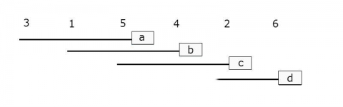
Step 1: After you calculate the LSD, you need to rank the means of the variable from lowest to highest.
| Treatment | Mean Yield |
|---|---|
| 3 | 115 |
| 1 | 117 |
| 5 | 121 |
| 4 | 124 |
| 2 | 128 |
| 6 | 135 |
Step 2: Calculate the differences between each mean to see if the difference is greater than the Least Significant Difference that you have already calculated. Hint: start with the highest and lowest means. If they are not significantly different, then none of the means between them are significantly different and then test ends here. If they are significant, continue by comparing the highest and second lowest and the second highest with the lowest. Continue until there are no more significantly different comparisons.
Step 3: You can visualize the differences between the means by writing the treatments horizontally.
3 1 5 4 2 6
Step 4: Underline the treatments that are not significantly different and ignore the lines that fall completely within the boundaries of other lines.
3 1 5 4 2 6
________
________
________
_____
Ex. 1: Supplement – LSD Results
Step 5: Use lowercase letters to label each line (Fig. 1).
Step 6: You can do this in table format as well, and this is what you will see in the R output.
| Treatment | Mean Yield |
|---|---|
| 3 | 115 a |
| 1 | 117 ab |
| 5 | 121 abc |
| 4 | 124 bc |
| 2 | 128 cd |
| 6 | 135 d |
Basically, if any means share a common letter, they are not significantly different!
Tukey’s Honestly Significant Difference
This procedure is essentially the same as the LSD, but this test takes into consideration the number of treatment means and utilizes the studentized range statistic to control for the Type I error. This is because the test statistic already limits the Type I error to 0.05.
To find the studentized range statistic (q) you need to know two values:
- p: The number of treatments for your group
- f: the number of error degrees of freedom
You can look up the corresponding q value using these values in a table online (Tukey’s test statistic). Once you have your q value, use the formula to calculate the HSD:
[latex]T_{\alpha} = q_{\alpha}(p,f)\sqrt{\frac{MSError}{r}}[/latex].
[latex]\textrm{Equation 6}[/latex] Formula for calculating studentized range statistic.
Here, r is the number of replications.
Once you calculate the HSD, you can use the same procedure as the LSD to figure out which means are significantly different.
Ex. 1: Supplement – LSD and HSD Resources
How to Calculate the Least Significant Difference (LSD).
Multiple Range Tests
Calculating Differences
The multiple range tests are extensions of the LSD. When there are several means, for example in the range between the highest and lowest, the LSD is multiplied by a factor depending on the number of means. For example, in the Duncan’s MRT, the LSD might be multiplied by 1.14 if we have 9 means counting the lowest up to the highest, or 1.08 if there are 4 in the range tested (for example first to fourth or third to sixth). We only declare the highest and lowest different if their difference exceeds 1.14 times the LSD.
We have described the method for testing various ranges of means but will rely on the computer to actually carry out a multiple range test (MRT). We have studied the method to understand how computer programs assign the same letter to ranges that are not significantly different. We will not, however, be laboring through all the calculations done by a computer in a MRT.
The main point about output from a MRT is to realize that means which share a common letter are not significantly different. Suppose after a MRT, our mean yields in an experiment with 6 treatments are listed as:
| Treatment | Mean Yield |
|---|---|
| 3 | 115 a |
| 1 | 117 ab |
| 5 | 121 abc |
| 4 | 124 bc |
| 2 | 128 cd |
| 6 | 135 d |
Definition
Multiple range tests protect better than LSD against Type I errors. The LSD discussed in the previous section works well for comparing selected means, usually adjacent means, in an experiment. The method is not useful for numerous comparisons or for comparing all the means. In an experiment with nine treatments there are 36 [9(9 – 1)/2] pairwise comparisons that can be made. If you were to use an LSD at the P = 0.05, then you might expect to make up to two Type I errors (0.05 x 36 = 1.8) among all the comparisons assuming there are no real differences among the treatments. The more comparisons you make, the more likely you are to make a mistake using the LSD, so we naturally try to limit our comparisons to those that are most important to us.
What if we want to make comparisons between all means? For example, what if we are comparing the grain yields of multiple corn hybrids? In this case, we can employ a Multiple Range Test. Such a test conservatively adjusts the required difference for significance to adjust for the distance between means in an array. The Honestly Significant Difference (HSD) is one of the tests for this purpose.
HSD
The HSD test, like the LSD test, determines the minimum significant difference (MSD) between means arrayed by magnitude (value). This difference is MSD = Q (S2/r)1/2, which is essentially the same formula as that for the LSD, except that Q contains a modified t-value times √2. For an experiment comparing only two means, LSD = HSD. When there are more than two means to be compared, the HSD controls the “experimentwise” Type I error rate to be 0.05. In other words, the HSD ensures that even with, say 15 treatment means, you will only falsely declare a difference to be significant in 5% of such experiments. However, with the HSD, individual comparisons are made at a P somewhat less than the stated probability level, so it is much more conservative than the LSD, which controls “comparisonwise” Type I error rate.
Appendix Table 6 has a column for error df on the left and separate columns for numbers of means compared (2 up to 20). The studentized range (Q) is then read from the table. For an experiment with the broadest comparison of six means with 24 df for the error mean square, Q = 4.373.
How to do HSD
The HSD multiple range test should be conducted in the following manner.
- Arrange means from highest to lowest.
- Compare the highest and lowest mean values. If the difference between the two values is not significant, draw a line beside the list connecting the two means or put the same letter next to each in the range. Conclude that there are no treatment differences.
- If the difference is significant, then the test continues. Compare the highest mean to the second-lowest mean and the lowest mean to the second-highest mean. If either difference is not significant, draw a line between the two means or put the same letter next to each in the range.
- When the difference between two means is declared not significant, then all means between the two compared are also declared not significant.
- Continue until all means have been compared directly or shown to be not significantly different within another comparison.
Contrasts
Contrasts are comparisons among several means. To this point, we have only been comparing pairs of treatment means, but often we need to compare several means. For example, suppose we have 3 nitrogen fertilizer treatments in a wheat experiment: manure, 25 kg N, and 50 kg N, the latter two being applied as urea. We would be interested in a comparison or contrast of average yield of the manure treatment vs. the two chemical fertilizer treatments. We want to test H0: (mean of treatment 1) = (mean of treatments 2 and 3). Just as with a contrast of two treatment means, we can use a t-test for testing whether a linear combination of the three treatment means is zero.
We can analyze contrasts with either a t-test (the next slide) or an F-test (described later in this lesson). With either test, we are comparing the differences between means or groups of means to the residual variation described by the standard error (in the F-test).
Test Equations
We test the linear combination:
[latex]L=\bar{Y}-\frac{\bar{Y}_1 + \bar{Y_2}}{2}[/latex].
[latex]\textrm{Equation 7}[/latex] Formula for calculating L value to test linear combination.
The t-test has form:
[latex]t=\frac{L}{S_L}[/latex].
[latex]\textrm{Equation 8}[/latex] Formula for calculating t value.
where:
L = the difference between the means of groups or groups of means,
SL = the standard error of the contrast.
Estimating Variance
The testing of contrasts of several means is somewhat more complicated than testing pairs of means because we need to estimate the variance of the linear combination, SL2. For our example,
[latex]S^2_L=(1)^2(\frac{S^{2}}{n_{1}}) + (-0.5)^2(\frac{S^{2}}{n_{2}}) + (-0.5)^2(\frac{S^{2}}{n_{3}})[/latex].
[latex]\textrm{Equation 9}[/latex] Formula for calculating variance of linear combination.
where:
[latex]S^{2}[/latex]= residual or error mean square,
[latex]n_{1}, n_{2}, n_{3}[/latex]= numbers of observations in treatments 1, 2, and 3, respectively.
Where did the “1” and “-0.5”s come from? By multiplying the corresponding means by these numbers, we calculate the same value as we did for  . In effect, we are finding the difference between
  and the mean of
  and
and  .
.
Linear Combination and Variance of Linear Contrast
Linear Combination
A linear combination of the treatment means is:
[latex]L= c_{1}\bar{Y_{1}} + c_{2}\bar{Y_{2}} + ... c_{t}\bar{Y_{t}} \textrm{ or} \textrm { L}=\sum_{i=1}^{t}c_{i}Y_{i}[/latex].
[latex]\textrm{Equation 10}[/latex] Formula for calculating linear combination, L, of contrasts.
where:
[latex]c_{t}[/latex]= contrast coefficient for treatment t,
[latex]\bar{Y_{t}}[/latex]= mean of treatment t.
Variance of the Linear Contrast
The variance of the linear contrast, each of whose treatments has r replications, is:
is
[latex]S^2_L=\sum_{i=1}^{t}c^2_i[/latex].
[latex]\textrm{Equation 11}[/latex] Formula for calculating variance of linear contrasts.
where:
[latex]S^2[/latex]= residual or error mean square,
[latex]c_{2}[/latex]= contrast coefficient for ith treatment mean
[latex]r[/latex]= number replications.
This formula for the estimated variance of a contrast makes sense because we are comparing t independent means. They are independent because of randomization in the experimental design. Each mean has an estimated variance (S2/r). Because the variance of a constant times a variable is the square of the constant times the variance of the variable, we have ci2 in the formula. In the simplest case, this reduces to: Sd2 = (S2/r) + (S2/r) for contrasting two treatment means [because ci2 = (1)2 or (-1)2]. The square root of this is the standard error for computing the LSD.
If in our wheat experiment, yields of the 3 treatments, each with 6 reps, are \bar{Y} = 70 bu/A, \bar{Y}_2 = 57 bu/A and \bar{Y}_3 = 64 bu/A, and the error mean square from the ANOVA is 78, what is the calculated t-value for the contrast?
Testing
The idea of contrasts is a straightforward extension of the idea of comparing two treatment means. In general, we make the contrast (L) among the treatment means and test the null hypothesis that the mean of the contrast is zero. If t = L/SL is larger than the critical t-value (for degrees of freedom in S2), we reject the null hypothesis. With 10 or more error df, the contrast is significant at the 0.05 probability level when L is over about 2 standard errors (SL) away from zero.
One more point is pertinent: we can also test the contrast with an F-test. Earlier we saw that a two-tailed t-test with k error degrees of freedom is the same as an F-test with one numerator and k denominator degrees of freedom because F = t2. F-tests for contrasts are often arranged into an ANOVA table so we can subdivide the treatment sum of squares into logical single-degree-of-freedom tests. We explore this further in the next section.
Planned F-Tests
Contrasts are planned comparisons and can be tested with F-tests. Perhaps the most powerful and useful method for comparing means is through contrasts, outlined in the previous section. They go beyond simple mean comparisons to answering specific questions about the treatment effect. They are especially useful in factorial experiments, where they allow the effect of one factor to be isolated and studied. In addition, contrasts can be used with quantitative variables (i.e., levels of fertilizer) to detect trends in the response of the experimental units. We outline in detail in this section how contrasts are set up, some of their properties, how they fit into an ANOVA table, and how they are tested with F-tests.
The first step in designing a contrast is to determine the questions that we desire to answer. This is the beauty of a contrast — it allows us to cut through all of the numbers and get back to the concepts for which we conducted the experiment!
For example, what questions would we want to answer with regard to the corn hybrid and population factorial experiment? Of course, we want to know whether higher plant populations improve corn yield. We also want to know whether the hybrids produce different yields.
Corn Example
Now let us further define these questions. We begin by specifying the population question. We ask two questions. First, how does the yield at 12.5 plants/m2 compare to the mean yield of 7.5 and 10.0 plants/m2? Secondly, does the yield for 7.5 plants/m2 differ from the yield for 10.0 plants/m2?
Among the corn hybrids we could compare the mean yield of hybrid C with the mean yield of hybrids A and B. We could then compare the yield of hybrid A with that of hybrid B.
These are examples of some of the logical contrasts which a researcher might want to test in his/her experiment. The contrasts chosen by a researcher will depend on the objectives for each experiment.
Population:
- 5.0 vs. 10.0 plants/m2
- 7.5 and 10.0 vs. 12.5 plants/m2
Hybrid:
- hybrid A vs. hybrid B
- hybrid A and B vs. hybrid C
Assigning Contrast Coefficients (1)
Contrast Coefficients are assigned +1 or -1 to compare equal-sized groups. The nuts and bolts behind a contrast is the generation of a difference. For example, in comparing the populations previously, what we are really doing is examining the numerical difference between the mean yield at 7.5 and 10.0 plants/m2. Therefore, the second step in a contrast is to generate this difference. This is accomplished by assigning different weights, called coefficients, to the nine treatment means produced by the experiment.
To determine the difference in mean yield between corn planted at 7.5 and 10.0 plants/m2, we need to compare two groups: the three treatment means produced at 7.5 plants/m2 and the three treatment means produced at 10.0 plants/m2. We will assign a coefficient of +1 to every treatment that is produced at 7.5 plants/m2 and a coefficient of -1 to every treatment produced at 10.0 plants/m2. We assign a coefficient of 0 to every treatment produced at 12.5 plants/m2, since we are not comparing that population in this contrast. As a reminder, in our numbering of treatments, the first three are 7.5 plants/m2 for hybrids A, B and C, treatments 4 to 6 are 10.0 and 7 to 9 are 12.5. The coefficients for our contrast of the nine treatments are:
| Contrast | 1 | 2 | 3 | 4 | 5 | 6 | 7 | 8 | 9 |
|---|---|---|---|---|---|---|---|---|---|
| 7.5 vs. 10.0 plants/m2 | +1 | +1 | +1 | -1 | -1 | -1 | 0 | 0 | 0 |
Assigning Contrast Coefficients (2)
What we are doing, then, is adding up all means produced at 7.5 plants/m2 and then subtracting all means produced at 10 plants/m2. The result is a difference which we will analyze. You might wonder why we use whole number coefficients instead of 1/3 and -1/3 since the contrast of interest is [latex]\large(\frac{\bar{Y}_1+\bar{Y}_2+\bar{Y}_3}{3})-(\frac{\bar{Y}_4+\bar{Y}_5+\bar{Y}_6}{3})[/latex]. It turns out that the F-ratio or t-test is the same whether we use the fractions or whole numbers, and it is easier to just use whole numbers. However, when calculating the actual difference being compared, it is important to use the correct fraction. In the example above, leaving out the denominator would give you the difference in totals rather than the difference in means. We can use totals to evaluate the significance of the contrast, but we need to use actual means when we estimate a treatment difference.
To determine the difference in mean yield between hybrid A and hybrid B, we follow the same procedure. We assign a coefficient of +1 to every treatment which includes hybrid A, and a coefficient of -1 to every treatment which includes hybrid B. We will assign a coefficient of 0 to every treatment which includes hybrid C, since that hybrid is not a part of this comparison. We assign the following coefficients to our nine treatments:
| Contrast | 1 | 2 | 3 | 4 | 5 | 6 | 7 | 8 | 9 |
|---|---|---|---|---|---|---|---|---|---|
| Hybrid A vs B | +1 | -1 | 0 | +1 | -1 | 0 | +1 | -1 | 0 |
Notice that it is imperative to pay close attention to how treatments are assigned.
Assigning Contrast Coefficients – Sums
Contrast coefficients are assigned weights which sum to zero. Comparing the yield produced at a population of 12.5 plants/m2 with the mean yield of 7.5 and 10.0 plants/m2 is a little trickier. Again, we are comparing two groups. This time, however, one of the groups is composed of two populations — 7.5 and 10.0 plants/m2 — while the other group is composed of only one population — 12.5 plants/m2. This changes the coefficients which must be assigned.
At first, it might appear that we should assign a coefficient of +1 to all treatments containing 7.5 or 10.0 plants/m2 and a coefficient of -1 to all treatments containing 12.5 plants/m2. This, however, would be wrong, for we would be comparing the sum of six treatment means (7.5 and 10.0 plants/m2) with the sum of only three treatment means (12.5 plants/m2).
Assigning Contrast Coefficients – Weighting
Instead, we assign a coefficient of +1 to all treatments containing 7.5 or 10.0 plants/m2 and a coefficient of -2 to all treatments containing 12.5 plants/m2. In doing this, we in effect weight the yields produced with 7.5 and 10.0 plants/m2 before comparing them with the yields produced at 12.5 plants/m2. We assign the following coefficients to our nine treatments:
| Contrasts | 1 | 2 | 3 | 4 | 5 | 6 | 7 | 8 | 9 |
|---|---|---|---|---|---|---|---|---|---|
| 7.5 vs. 10.0 plants/m2 | +1 | +1 | +1 | -1 | -1 | -1 | 0 | 0 | 0 |
| 12.5 vs. 7.5 | +1 | +1 | +1 | +1 | +1 | +1 | -2 | -2 | -2 |
Notice that our contrast coefficients are balanced in that they sum to zero. This is a characteristic of contrast coefficients when treatments are equally replicated. Also notice that they are directly proportional to the fractional coefficients (+1/6, +1/6, +1/6, +1/6, +1/6, +1/6, -1/3, -1/3, -1/3) which result from the contrast of the (mean of 7.5 or 10.0 plants/m2) vs. (mean of 12.5 plants/m2).
Assigning Contrast Coefficients – Comparison
A good rule of thumb to remember when comparing groups containing different numbers of treatment means is this: assign each member of the first group a coefficient equal to the number of treatments in the second group. Then assign each member of the second group the negative value of the number of treatments in the first group.
We treat the comparison of the yield of hybrid C and the mean yield of hybrids A and B in the same way. We assign a coefficient of +1 to all treatments containing hybrids A or B and a coefficient of -2 to all treatments containing hybrid C.
| Contrast | 1 | 2 | 3 | 4 | 5 | 6 | 7 | 8 | 9 |
|---|---|---|---|---|---|---|---|---|---|
| Hybrid A vs. B | +1 | -1 | 0 | +1 | -1 | 0 | +1 | -1 | 0 |
| Hybrids C vs. A & B | +1 | +1 | -2 | +1 | +1 | -2 | +1 | +1 | -2 |
Independence of Comparisons
Orthogonal comparisons have the property of independence.
Two rules must be followed in order for a set of contrasts to be independent of each other. These are for treatments with equal numbers of reps, which is the usual case when there is no missing data in an experiment.
Rule 1
The sum of the coefficients in each contrast must equal zero.
| Contrast | 1 | 2 | 3 | 4 | 5 | 6 | 7 | 8 | 9 |
|---|---|---|---|---|---|---|---|---|---|
| Hybrid A vs. B | +1 | -1 | 0 | +1 | -1 | 0 | +1 | -1 | 0 |
Rule 2
The sum of the product of the corresponding coefficients of any two contrasts must equal zero.
| Contrast | 1 | 2 | 3 | 4 | 5 | 6 | 7 | 8 | 9 |
|---|---|---|---|---|---|---|---|---|---|
| Hybrid A vs. B | +1 | -1 | 0 | +1 | -1 | 0 | +1 | -1 | 0 |
| Hybrids C vs. A & B | +1 | +1 | -2 | +1 | +1 | -2 | +1 | +1 | -2 |
| Product of contrasts | +1 | -1 | 0 | +1 | -1 | 0 | +1 | -1 | 0 |
Non-orthogonal Contrasts
It is possible and sometimes even desirable to make a set of contrasts that are not orthogonal. The advantage of using an orthogonal set is that if the sums of squares for each contrast are added together, the sum is equal to the sum of squares for treatments in the ANOVA. This characteristic can be useful when performing calculations. It also provides a way to efficiently use all the information available for treatment comparisons. Interpretation of a set of contrasts is also more straight forward when they are independent.
For 4 treatments, are the following pairs orthogonal contrasts?
Contrast Sums of Squares
Each contrast has a sum of squares in the ANOVA.
Each contrast produces a sum of squares which is calculated using treatment means and coefficients. The F-ratio is the square of the calculated t-value L/SL. The formula for the contrast sum of squares is
[latex]\textrm{Contrast SS} =\frac{r(\sum{c\bar{Y}})^2}{\sum{}c^{2}}[/latex].
[latex]\textrm{Equation 12}[/latex] Formula for calculating contrast sum of squares.
where:
[latex]c[/latex]= contrast coefficient,
[latex]r[/latex]= number replicates.
The contrast SS has 1 df, so the Contrast MS = Contrast SS. Basically, t2 = F (the variance ratio). So, the square of the t-value you calculated earlier is equal to the Contrast MS/ Residual Mean Square (RMS).
Calculating Contrast SS
The sum of squares for comparison of yields produced at 7.5 and 10.0 plants/m2 is calculated as follows. Of course, the computer calculates this for you, but it is good to see this calculation to know how much work it saves you!
[latex]\text{SS(7.5 vs. 10 plants} /m^2)= \frac{3*((1) 150.6 + (1) 149.5) + (1) 135.8 + (-1) 136.0 + (-1) 159.0 + (-1) 152.1 + (0) 169.1 + (0) 124.5 + (0) 89.0)}{(1^2 + 1^2 + 1^2 + (-1)^2 + (-1)^2 + (-1)^2 + 0 + 0 + 0)} = \frac{3*(-11.2)^2}{6} = 62.72[/latex].
Corn Population Example
The results can be arranged in the same manner as an ANOVA table. The sums of squares for all four contrasts are therefore:
| Contrast | df | SS | MS | F | F crit (P = 0.05) |
|---|---|---|---|---|---|
| 7.5 vs. 10.0 plants/m2 | n/a | 62.72 | n/a | n/a | n/a |
| 7.5 and 10.0 vs. 12.5 plants/m2 | n/a | 107.925 | n/a | n/a | n/a |
| hybrid A vs. B | n/a | 5.021 | n/a | n/a | n/a |
| hybrid A and B vs. C | n/a | 1.564 | n/a | n/a | n/a |
| error | n/a | 563.611 | n/a | n/a | n/a |
The sum of squares for error is calculated as in the ANOVA with all treatment sums of squares, not just those for the 4 contrasts, removed.
Mean Square
Contrasts have 1 df, so contrast MS = contrast SS.
The mean square for each contrast and the error is calculated by dividing the sum of squares by the degrees of freedom. Each contrast has one degree of freedom. Therefore, the mean square for each contrast is equal to its sum of squares:
| Contrast | df | SS | MS | F | F crit (P = 0.05) |
|---|---|---|---|---|---|
| 7.5 vs. 10.0 plants/m2 | 1 | 4.726 | 4.726 | n/a | n/a |
| 7.5 and 10.0 vs. 12.5 plants/m2 | 1 | 107.925 | 107.925 | n/a | n/a |
| hybrid A vs. B | 1 | 5.021 | 5.021 | n/a | n/a |
| hybrid A and B vs. C | 1 | 1.564 | 1.564 | n/a | n/a |
| error | 18 | 563.611 | 31.312 | n/a | n/a |
Compare this result with the ANOVA table calculated in R Exercise 1 in Chapter 9 on Two Factor ANOVAs. Notice that the contrast df and SS for population and for hybrid sum to those found in the ANOVA table (with some small rounding errors). There is one portion of the ANOVA from Chapter 9 missing, though, the interaction between the treatments. Orthogonal contrasts could also be constructed for the interaction, but we will not do that here.
F-Tests
To calculate the F-value for each contrast, the mean square for each contrast is divided by the mean square error:
| Contrast | df | SS | MS | F | F crit (P = 0.05) |
|---|---|---|---|---|---|
| 7.5 vs. 10.0 plants/m2 | 1 | 4.726 | 4.726 | 0.15 | n/a |
| 7.5 and 10.0 vs. 12.5 plants/m2 | 1 | 107.925 | 107.925 | 3.45 | n/a |
| hybrid A vs. B | 1 | 5.021 | 5.021 | 0.16 | n/a |
| hybrid A and B vs. C | 1 | 1.564 | 1.564 | 0.05 | n/a |
| error | 18 | 563.611 | 31.312 | n/a | n/a |
F-Test Critical Value
The contrast for each F-value is then compared with the critical F-value for the desired level of significance (F with 1 numerator and 18 denominator df).
| Contrast | df | SS | MS | F | F crit (P = 0.05) |
|---|---|---|---|---|---|
| 7.5 vs. 10.0 plants/m2 | 1 | 4.726 | 4.726 | 0.15 | 0.70 |
| 7.5 and 10.0 vs. 12.5 plants/m2 | 1 | 107.925 | 107.925 | 3.45 | 0.08 |
| hybrid A vs. B | 1 | 5.021 | 5.021 | 0.16 | 0.69 |
| hybrid A and B vs. C | 1 | 1.564 | 1.564 | 0.05 | 0.83 |
| error | 18 | 563.611 | 31.312 | n/a | n/a |
Notes To Instructors
This lesson will focus on the calculating of contrasts using the R software, it is assumed that we already how to calculate contrast coefficients in order to make specific comparisons. A brief overview of how to assign contrast coefficients can be found in the supplementary materials at the end of the activity.
Ex. 2: Getting Ready
R Code Functions
- read.csv()
- as.factor()
- list()
- aov()
- matrix()
- split()
- summary()
- contrasts()
- interaction()
The Premise
The previous LSD and HSD test indicate that the means of Population are not significantly different. However, the LSD test shows the average yield of Hybrid A and B is different than that of Hybrid C. If we want to further to explore specific means or group of means comparisons for variables Population and Hybrid, contrast is the best way to do this. So, continuing from the same experiment of planting 3 hybrids at 3 planting densities, you now wish to make specific comparisons between hybrids and comparisons between populations.
Activity Objectives
Use R to calculate specific contrasts that you choose to run.
Ex. 2: Read Data
Suppose we want to create two contrasts for main effect of Population, we named:
- C1: compare the yields of two populations 7.5 and 10 plants/m2.
- C2: compare the yield produced at a population of 12 plants/m2 with the mean yield of populations 7.5 and 10 plants/m2.
If you have picked up from the previous activity, you will not need to run the ANOVA again, but if you are starting fresh with this assignment, use the following code to read in the data set and run the two-factor ANOVA. Be sure to have Population as a factor in R before you run your analysis or you will not have the appropriate number of degrees of freedom for Population.
corn<-read.csv(”exercise.10.2.data.csv”,header=T)
Ex. 2: Contrast Coefficients
corn$Population <- as. factor(corn$Population)
Population <- corn$Population
cornaov<- aov(Yield ~ Population*Hybrid, data=corn)
Summary(cornaov)
Df Sum Sq Mean Sq F value Pr(>F)
Population 2 9.18 4.588 2.114 0.1498
Hybrid 2 12.18 6.342 2.922 0.0796
Population:Hybrid 4 29.30 7.325 3.375 0.0316
Residuals 18 39.07 2.170
—
Signif. codes: 0 ‘***’ 0.001 ‘**’ 0.01 ‘*’ 0.05 ‘.’ 0.1 ‘ ‘ 1
Next, make a matrix with the two sets of contrast coefficients. Then set the “contrasts” attribute of factor Population. For more information on how to calculate the contrast coefficients, see the supplementary materials for this activity. The following code will spell out the desired contrast and calculate it for us.
contrasts(corn$Population) <- matrix(c(1,-1,0,-1,-1,2), nrow = 3)
contrasts(corn$Population)
[,1] [,2]
30 1 -1
40 -1 -1
50 0 2
Ex. 2: Contrast Coefficients – Output
In the output, we have generated a matrix of contrast coefficients comparing 7.5 plants /m2 to 10 plants/m2 in column 1 and the mean of 7.5 and 10 compared to 12.5 plants/m2 in column 2. Remember, always double check that your contrasts (columns here) add up to 0! Next, we run the ANOVA again and this time we use the ‘split’ and ‘list’ function to add the contrasts we are interested in to the ANOVA.
Pop.model <- aov(Yield ~ Population*Hybrid, data = corn)
summary.aov(Pop.model, split = list(Population = list(”7.5 vs 10” = 1, “12.5 vs 7.5+10” =2)))
Df Sum Sq Mean Sq F value Pr(>F)
Population 2 9.18 4.588 2.114 0.14975
Population: 7.5 vs 10 1 0.24 0.238 0.110 0.74434
Population: 12.5 vs 7.5+10 1 8.94 8.939 4.118 0.05748 .
Hybrid 2 12.68 6.342 2.922 0.07962 .
Population:Hybrid 4 29.30 7.325 3.375 0.03156 *
Population:Hybrid: 7.5 vs 10 2 3.04 1.521 0.701 0.50931
Population:Hybrid: 12.5 vs 7.5+10 2 26.26 13.130 6.049 0.00978 **
Residuals 18 39.07 2.170
—
Signif. codes: 0 ‘***’ 0.001 ‘**’ 0.01 ‘*’ 0.05 ‘.’ 0.1 ‘ ’ 1
The results show that the both contrasts “7.5 vs 10” and “12.5 vs 7.5 + 10” on the main effect of Population are not significant with P = 0.7444 and P = 0.057, respectively. And also that the second contrast on Population has a significant interaction with Hybrid, F(1,18) = 6.409, P = 0.01.
Ex. 2: Contrasts for Hybrid Effect
Let’s switch to construct contrasts for main effect of Hybrid. Similarly, we named,
- C3: compare the mean yield between hybrid A and hybrid B,
- C4: compare the yield of hybrid C and the mean yield of hybrids A and B.
The R code for calculating above two contrasts would be the same as the ones of Population.
contrasts(corn$Hybrid) <- matrix(c(1,-1,0,-1,-1,2), nrow = 3)
contrasts(corn$Hybrid)
[,1] [,2]
A 1 -1
B -1 -1
C 0 2
Hybrid.model <- aov(Yield ~ Population*Hybrid, data = corn)
summary.aov(Hybrid.model, split = list(Hybrid = list(”A vs B” = 1, “C vs A+B” = 2)))
Df Sum Sq Mean Sq F value Pr(>F)
Population 2 9.18 4.588 2.114 0.1498
Hybrid 2 12.68 6.342 2.922 0.0796 .
Hybrid: A vs B 1 1.00 0.999 0.460 0.5062
Hybrid: C vs A+B 1 11.69 11.685 5.384 0.0323 *
Population:Hybrid 4 29.30 7.325 3.375 0.0316 *
Population:Hybrid: A vs B 2 13.53 6.765 3.117 0.0688 .
Population:Hybrid: C vs A+B 2 15.77 7.886 3.633 0.0473 *
Redsiduals 18 39.07 2.170
—
Signif. codes: 0 ‘***’ 0.001 ‘**’ 0.01 ‘*’ 0.05 ‘.’ 0.1 ‘ ’ 1
Ex. 2: Interaction
We can see that the yield of Hybrid A is not different from that of Hybrid B with P = 0.5062. However, the average yield of Hybrid A and B is different than that of Hybrid C with P = 0.0323. Now we know that if say, Hybrid C was a standard check variety, it would be different than the other two varieties in your trial, but Hybrid A and Hybrid B are not really different in terms of yield. You’ll want to take information like this into consideration if you are trying to decide which Hybrids to keep in your breeding program.
Let’s say we think that a particular hybrid is affected by Population because we saw evidence of it in the ANOVA or the interaction plot. In this example, we can see that Hybrid C is affected by Population. To figure out which Populations differ in yield when growing Hybrid C, we need to make two contrasts: 7.5 vs. 10 and 10 vs. 12.5. To do this in R, we first have to compute a factor which represents the interaction of Population and Hybrid.
We named the new interaction factor as “P.H”, which has 9 levels, ordered from 7.5.A to 12.5.C.
corn$P.H <- interaction(corn$Population, corn$Hybrid)
corn$P.H
[1] 7.5.A 7.5.A 7.5.A 7.5.B 7.5.B 7.5.B 7.5.C 7.5.C 7.5.C 10.A 10.A 10.A 10.B 10.B 10.B 10.C
[17] 10.C 10.C 12.5.A 12.5.A 12.5.A 12.5.B 12.5.B 12.5.B 12.5.C 12.5.C 12.5.C
Levels: 7.5.A 10.A 12.5.A 7.5.B 10.B 12.5.B 7.5.C 10.C 12.5.C
Ex. 2: Compare Yield – 7.5 vs 10
Next we set the contrast coefficients to compare the yield difference between 7.5 and 10 for Hybrid C.
contrasts(corn$P.H) <- c(0,0,0,0,0,0,1,-1,0)
contrasts(corn$P.H)
[,1] [,2] [,3] [,4] [,5] [,6] [,7] [,8]
7.5.A 0 -0.33333333 -0.33333333 -0.33333333 -0.33333333 -0.09763107 -0.5690356 -0.33333333
10.A 0 -0.08333333 -0.08333333 -0.08333333 -0.08333333 -0.73151455 -0.5648479 -0.08333333
12.5.A 0 0.91666667 -0.08333333 -0.08333333 -0.08333333 -0.02440777 -0.1422589 -0.08333333
7.5.B 0 -0.08333333 0.91666667 -0.08333333 -0.08333333 -0.02440777 -0.1422589 -0.08333333
10.B 0 -0.08333333 -0.08333333 0.91666667 -0.08333333 -0.02440777 -0.1422589 -0.08333333
12.5.B 0 -0.08333333 -0.08333333 -0.08333333 0.91666667 -0.02440777 -0.1422589 -0.08333333
7.5.C 0 -0.08333333 -0.08333333 -0.08333333 -0.08333333 0.47559223 0.3577411 -0.08333333
10.C 1 -0.08333333 -0.08333333 -0.08333333 -0.08333333 0.47559223 0.3577411 -0.08333333
12.5.C -1 -0.08333333 -0.08333333 -0.08333333 -0.08333333 -0.02440777 -0.1422589 0.91666667
The contrasts get stored as attributes of the factor P.H. So when we run a new ANOVA they will get applied automatically. The contrast matrix has eight sets of contrasts. We are only interested in the first one and ignore the rest of them. Therefore, the argument of list is “label of contrast = 1”.
Interaction.model <- aov(Yield ~ P.H, data = corn)
summary.aov(Interaction.model, split = list(P.H = list(”7.5 vs 10, Hybrid C” = 1)))
DF Sum Sq Mean Sq F value Pr(>F)
P.H 8 51.16 6.395 2.946 0.0271
P.H: 7.5 vs 10, Hybrid C 1 1.53 1.530 0.705 0.4121
Residuals 18 39.07 2.170
—
Signif. codes: 0 ‘***’ 0.001 ‘**’ 0.01 ‘*’ 0.05 ‘.’ 0.1 ‘ ’ 1
Ex. 2: Compare Yield – 10 vs 12.5
The same R code can be applied for calculating the contrast 10 vs. 12.5 except changing the contrast coefficients of factor P.H and the label in list.
contrasts(corn$P.H) <- c(0,0,0,0,0,0,1,-1,0)
contrasts(corn$P.H)
[,1] [,2] [,3] [,4] [,5] [,6] [,7] [,8]
7.5.A 0 -0.33333333 -0.33333333 -0.33333333 -0.33333333 -0.33333333 -0.09763107 -0.5690356
10.A 0 -0.08333333 -0.08333333 -0.08333333 -0.08333333 -0.08333333 -0.73151455 -0.5648479
12.5.A 0 0.91666667 -0.08333333 -0.08333333 -0.08333333 -0.08333333 -0.02440777 -0.1422589
7.5.B 0 -0.08333333 0.91666667 -0.08333333 -0.08333333 -0.08333333 -0.02440777 -0.1422589
10.B 0 -0.08333333 -0.08333333 0.91666667 -0.08333333 -0.08333333 -0.02440777 -0.1422589
12.5.B 0 -0.08333333 -0.08333333 -0.08333333 0.91666667 -0.08333333 -0.02440777 -0.1422589
7.5.C 0 -0.08333333 -0.08333333 -0.08333333 -0.08333333 0.91666667 -0.02440777 -0.1422589
10.C 1 -0.08333333 -0.08333333 -0.08333333 -0.08333333 -0.08333333 0.47559223 0.3577411
12.5.C -1 -0.08333333 -0.08333333 -0.08333333 -0.08333333 -0.08333333 0.47559223 0.3577411
Interaction.model <- aov(Yield ~ P.H, data = corn)
summary.aov(Interaction.model, split = list(P.H = list(”7.5 vs 10, Hybrid C” = 1)))
DF Sum Sq Mean Sq F value Pr(>F)
P.H 8 51.16 6.395 2.946 0.0271
P.H: 7.5 vs 10, Hybrid C 1 1.53 1.530 0.705 0.4121
Residuals 18 39.07 2.170
—
Signif. codes: 0 ‘***’ 0.001 ‘**’ 0.01 ‘*’ 0.05 ‘.’ 0.1 ‘ ’ 1
The results of the two contrasts show that the yields of Hybrid C are the same for the 7.5 and 10 populations with F(1, 18) = 0.705, P = 0.4121 and differ from the yield at the 12.5 population with F(1, 18) = 10.602, P = 0.0044. Therefore it is reasonable to assume that Hybrid C is impacted by a higher planting density than the other two Hybrids.
Ex. 2: Review
Review Questions
- What have we learned from this lesson?
- How do LSDs and HSDs help make selection decisions?
| R Code Glossary | |
|---|---|
| read.csv(“”) | Read in a .csv file. Remember to include if it has a header or not. |
| aov(y ~ A + B + A:B, data=mydataframe) | Perform a 2-factor analysis of variance on an R object. Can also write as aov (y~A*B, data = mydataframe). |
| summary() | Returns the summary of an analysis |
| as.factor(mydataframe$variable) | Changes a variable within an R object to a factor variable. An example is when you have variables designated with numbers, but they are meant to be categorical variables, so you use this function to tell R that. |
| matrix(,nrow=) | Creates a matrix of a given size. You can specify a vector you already have or enter your own. |
| contrasts(x) | Sets contrasts matrix, x is a factor. In this activity, we specify a factor within a data frame ex: (corn$Population). |
| list() | A generic vector containing other objects. |
| split() | Splits a character vector. |
| interaction(…) | Computes a factor representing the interaction of the given factors. |
Ex. 2: Supplement – Decide Comparison(s)
When assigning contrast coefficients, you first need to decide what comparison(s) you wish to make. In the activity example, we compare planting densities of 7.5 and 10 plants/m2, and we make another comparison of 12.5 plants/m2 versus the mean of 7.5 and 10 plants/m2. For this first comparison, we will assign a coefficient of +1 to every treatment of 7.5 and -1 for every treatment of 10. The treatments of 12.5 are not included in this comparison, so every treatment with 12.5 will have a coefficient of 0.
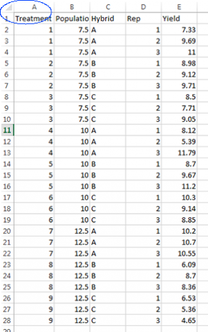
So, what are the treatments? If you go back to the datasheet, you will see that there is a column labeled ‘treatment’, and it lists treatments 1-9. Each treatment represents each Hybrid and Population combination, and each treatment is listed 3 times for the 3 replications (Fig. 2). If you have to come up with your own contrast coefficients, it is a good idea to clearly label your treatments for easy reference when assigning coefficients.
Ex. 2: Supplement – Assign Coefficients
Now that we have defined the comparisons and labeled our treatments, it is time to assign the coefficients. For 7.5 vs. 10 plants/m2 we assign a +1 for each treatment of 7.5 plants and -1 for each assignment of 10 plants. Remember, 12.5 is not included in this comparison so any 12.5 plant treatments are given a 0. What is happening here is we are subtracting the mean of the 10 plants/m2 from the mean of the 7.5 plants per acre and we will analyze the difference between the two for this contrast. You could use a coefficient of +1/3 instead of +1 since you have 3 treatments and while the F-test will turn out the same you would have to use the correct fraction to get the correct answer. This can be tricky with more complicated contrasts so you may just want to stick to whole numbers for your coefficients.
| Treatment # | 1 | 2 | 3 | 4 | 5 | 6 | 7 | 8 | 9 |
|---|---|---|---|---|---|---|---|---|---|
| Contrast 7.5 vs. 10.0 | +1 | +1 | +1 | -1 | -1 | -1 | 0 | 0 | 0 |
Following this same procedure, we can compare 12.5 plants/m2 to the mean of 7.5 and 10 plants/m2. This time we do not assign a coefficient of -1 to 7.5 and 10 and +1 to 12.5 because then we would be comparing the sum of 6 treatment means to only 3 treatment means. To deal with this we weight the means by assigning -1 to 7.5 and 10 and +2 to 12.5 plants/m2 to make this an even comparison.
| Treatment # | 1 | 2 | 3 | 4 | 5 | 6 | 7 | 8 | 9 |
|---|---|---|---|---|---|---|---|---|---|
| Contrast 7.5 vs. 10.0 | +1 | +1 | +1 | -1 | -1 | -1 | 0 | 0 | 0 |
| 7.5 and 10 vs. 12.5 | +1 | +1 | +1 | -1 | -1 | -1 | 2 | 2 | 2 |
You can use the same procedure to design any comparison that you wish to make.
Trend Comparisons
Trend comparisons are contrasts among quantitative treatments. The contrasts performed so far in this lesson have been class comparisons — they determine differences between different qualitative traits or levels of treatments. Class comparisons are by themselves adequate when we are working with qualitative data. For example, we would use qualitative comparisons when comparing different tillage implements or different kinds of fertilizer. The qualitative comparison is also appropriate for comparing corn hybrids, as we just did.
When we are working with quantitative data, however, we should not be content with class comparisons alone! For example, when comparing different rates of fertilizer, we want to know how the crop responds to extra fertilizer:
- Does the crop respond positively to every additional increment of fertilizer?
- Is there an optimum amount of fertilizer beyond which the crop actually responds negatively?
- If we can answer these questions, then we vastly expand our understanding of the yield response to applied fertilizer.
Whereas the class comparisons are useful when looking at discrete variables, the trend comparison can indicate responses of continuous variables. For instance, we found the response at 0, 25, and 50 kg/ha.
- What would happen if there were 35 kg N?
Linear Trend
A linear trend contrast is a comparison of high population with low
The response of corn yield to increasing population can be described using trend comparisons. Yield may increase with every increase in population (Fig. 3). The numbers along the left axis correspond to the coefficients that would be assigned to each population in a trend comparison.
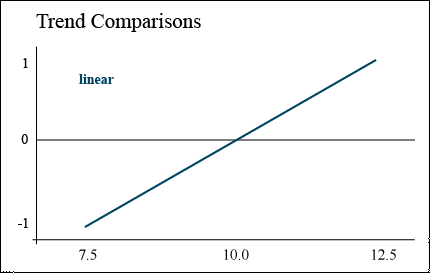
In this case, the contrast is comparing the difference between the highest and lowest populations, assuming a straight line between them. This is known as a linear trend.
Quadratic Trend
A quadratic trend comparison tests for curvature
Alternately, corn yield may increase with population up to 10.0 plants/m2, but then decrease when the population is increased to 12.5 plants/m2. Corn is particularly sensitive to available sunlight — a population which is too high will cause excessive shading and barrenness. This response trend is illustrated by the parabolic response curve (Fig. 4).
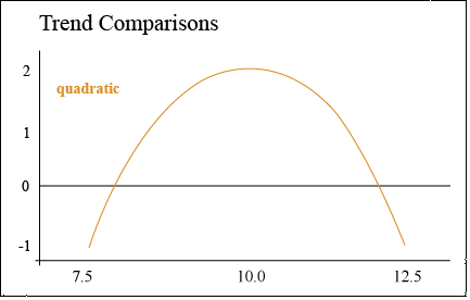
In this case, the contrast compares the middle plant population to the sum of the high and low population to determine whether there is a significant peak in yield. In other words, we are determining whether the population is optimal at 10.0.
Contrast Weights
Contrasts can be used to ascertain the order or the equation that best describes the relationship between a dependent variable such as yield and a quantitative variable such as population. You can use orthogonal polynomial contrasts for quantitative variables for polynomial models up to t – 1 terms; i.e. the maximum order you can explore with the contrasts is one less than the total number of levels for the quantitative treatment. In our example, we are constrained to and really only interested in computing linear (1st order) and quadratic (2nd order) contrasts. These will tell us if the response is a straight line or has some curvature (i.e. nonlinear).
The coefficients to be used with each comparison are shown (Table 21). In the case of both the linear and quadratic trend, these coefficients will test either an increasing or a decreasing trend. In other words, if yield decreased with population, or was actually lowest at 10 plants/m2, the coefficients below would detect those trends as well.
| Contrast | 1 | 2 | 3 | 4 | 5 | 6 | 7 | 8 | 9 |
|---|---|---|---|---|---|---|---|---|---|
| Linear | -1 | -1 | -1 | 0 | 0 | 0 | +1 | +1 | +1 |
| Quadratic | -1 | -1 | -1 | 2 | 2 | 2 | -1 | -1 | -1 |
Coefficients similar to these can be created for cubic, quartic, etc., trends if there are more plant population treatments. Tabulations of coefficients for different levels of treatments can be found under the Orthogonal tab in the Statistical Tables workbook.
Data Analysis
The two comparisons of the corn population experiment are tested using the same procedure as for class comparisons. The sum of squares and mean square for each comparison is calculated, and then the mean square for each comparison is subjected to the F-test. The results are shown in Table 5:
| Contrast | df | SS | MS | F | F crit (p = 0.05) |
|---|---|---|---|---|---|
| linear | 1 | 4.726 | 39.15 | 1.25 | 4.41 |
| quadratic | 1 | 107.925 | 37.5015 | 1.20 | |
| error | 18 | 563.611 | 31.312 |
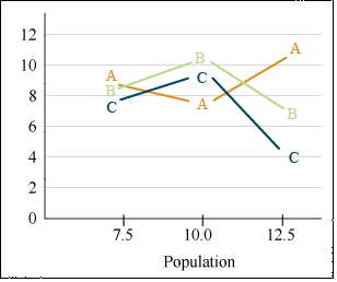
Viewing the data in Fig. 5 helps to explain why the linear and quadratic trends did not show significance here. There are hints of both types of trend (linear and quadratic) for each population, but no clear trend for all hybrids is obvious.
Hybrids B and C show an optimal population at 10.0, while hybrid A actually performed worst at 10.0. This discussion on linear and quadratic contrasts for trend analysis completes our study of contrasts as mean separation techniques.
Summary
Comparing Means
- LSD for adjacent pairs or comparison with check cultivar
- HSD for better Type I Error control
- Multiple range tests also protect better than LSD
LSD
- Equals t standard errors of a difference
- Is the most commonly used method for comparing means
Contrasts
- Are planned comparisons
- Tested with t-test or F-test
- LSD is the simplest case
- Coefficients sum to zero if equal replication
Orthogonal Contrasts
- Independent comparisons
- Partition the treatment sum of squares
Trend Analysis
- Can be done with contrasts
- Useful for quantitative data
- Provides response curve
- Will be done with regression in this chapter and the one on Randomized Complete Block Design
How to cite this chapter: Moore, K., R. Mowers, M.L. Harbur, L. Merrick, A. A. Mahama, & W. Suza. 2023. Mean Comparisons. In W. P. Suza, & K. R. Lamkey (Eds.), Quantitative Methods. Iowa State University Digital Press.
Qualitative variables are those to which no meaningful numerical values can be assigned. Compare quantitative.
A conservative test is one that does not indicate significance unless the probability of chance occurrence is very small. There is less chance for indicating a significant difference when something is truly not different.
Quantitative variables are numerical in nature. They can be ranked along some scale of measurement which has inherent meaning. Compare qualitative.
A method used to determine the response relationship of data. This method determines whether data is linear (form y=ax+b), parabolic (y=ax2+bx+c), or higher order.
an equation of a form y=ax+b, y=ax^2+bx+c, or higher order.
a multiplicative numerical value, factor, or weighing factor in some equation. They may be used to weigh different treatments in a contrast or be a factor in a polynomial equation.
The response for different treatments can be determined by separating the contrasts or making them independent. Another term for them is calling them orthogonal. The differences can be compared between varieties and populations from the same experiment. To be independent, any interaction between the treatments must be removed. Thus, differences of variety or population may be compared without concern for interaction with the other effect.
Orthogonality means that the contrasts ask independent questions. There isn't any overlap in the information for comparison of treatment means.
Statistical comparison done between groups of different traits, such as hybrids, or between discrete levels of application, such as populations or fertilizer rates.
