
Chapter 3: Central Limit Theorem, Confidence Intervals, and Hypothesis Tests
Ron Mowers; Dennis Todey; Kendra Meade; William Beavis; Laura Merrick; Anthony Assibi Mahama; and Walter Suza
In Chapter 2 on Distributions and Probability, we saw some examples of data distributions, especially the normal distribution, and learned to make probability statements from that distribution. In this unit, we see that sample means from a normal distribution are also distributed normally, but with variance reduced by a factor of n (the number of observations in the sample). We also tie these ideas to the scientific method of chapter 1 on Basic Principles by learning how to test hypotheses.
- Sample averages from a normal distribution are normally distributed.
- The central limit theorem.
- How to form confidence intervals for the mean of a normal distribution.
- How to create and test a hypothesis.
Distribution of Sample Averages
Averages of Samples
Averages of samples from a normal distribution also follow a normal distribution. Often we wish to estimate the mean of a population. We use sample averages to estimate the mean of a population of interest. What about these sample means — how can they be described? A set of sample means comprises its own population, which surprisingly approaches the normal distribution about the population mean.
The idea is this: suppose we start with a full normal distribution, take a sample of 10 observations, then compute the sample average. Then we take a second sample of 10 observations and again compute its sample mean. We repeat this process many times.
Extreme Sample Mean Values
When we try to produce a distribution using sample means of just a few individuals, we notice that the curve is flatter and wider than if more individuals are in the sample. If an extreme (far from the mean) value is included in the sample, then it will have a large proportional effect in widening the distribution if the sample size is small. As we increase the number of individuals in the sample, the distribution for sample means grows narrower and taller. The effect of extreme values is diluted by the larger number of values closer to the population mean.
Probability Distribution
Click here to download a file that examines the distribution of sample means: Distributions [XLS]
The probability distribution for a set of sample means, like the probability distribution for the actual population, can be described with only two measurements: the mean, and the standard error of the mean. The mean, μx, is the mean for the population of the sample means. The standard error of the mean, or standard deviation of sample means, is denoted by σx. It describes the standard deviation of individual sample means around the population mean for the set, and is estimated by:
[latex]S^2_{\small\bar{x}}[/latex] = [latex]\dfrac{S^2}{n}[/latex]
[latex]\text{Equation 1}[/latex] Formula for computing the standard error of the mean,
where:
[latex]S^2_{\small\bar{x}}[/latex] = variance of sample mean, [latex]\bar{x}[/latex]
[latex]{S^2}[/latex] = variance of the sample
[latex]{n}[/latex] = number of values in the sample
The important thing to see from this formula is the relationship of the variance of sample means to the original variance of the sample — it is reduced by a factor of n. Sample means have less variance than do the original observations. The reduction factor is the sample size n.
Whenever we try to describe a population based on a sample, we must ask: how well does our sample mean represent the actual population mean, μ? We will answer this question when we study confidence intervals for the mean.
Standard Error of the Mean
Just as the standard deviation of the population is calculated as the square root of the population variance, the standard error of the mean, SE, is calculated as the square root of the sample variance, divided by the number of observations:
[latex]SE = \sqrt{\dfrac{^{S}}{n}}[/latex]
[latex]\text{Equation 2}[/latex] Formula for computing SE,
where:
[latex]{SE}[/latex] = standard error of mean
[latex]{S^2}[/latex] = sample variance
[latex]{n}[/latex] = number of values in the sample
The standard error of the mean (SE) is commonly used to tell how much sample means fluctuate from sample to sample. Usually, we take a set of individuals from a population and calculate the mean of them to try to estimate the population mean. How that mean compares to the population mean is assessed using the standard error.
Central Limit Theorem
Normal Distribution
Interestingly enough, means of samples from even a non-normal distribution can be normally distributed. This is the gist of what is called the “Central Limit Theorem.” It states that when we draw simple random samples of size n from any distribution, the sample means become approximately normally distributed with mean μ and variance σ2/n (for large sample sizes).
Naturally, one question that comes to mind is, “How large must n be for the normal approximation to hold?” This depends on how similar to a normal distribution our original distribution is. If the original distribution is a normal one, the sample means are always normal, no matter how small the sample (even individual values are normally distributed). As the original distribution becomes less and less like the bell-shaped curve, sample sizes need to be larger to have sample averages nearly normally distributed.
Data Distributions
In the chapter 2 on Distributions and Probability, we looked at various types of data distributions including the normal distribution. Many groups of data are not normally distributed, but some closely approximate it. We will look at one of those and do some work with those data.
We have looked at monthly temperature data in chapter 2 and assumed that they were from a normal distribution. Now we will test whether that data is close to a normal distribution. This is both a review of some concepts from chapter 2 and some new methods for testing and working with the normal distribution.
The z-statistic in a normal distribution in essence standardizes the value. The standardized distribution has a mean of zero and a standard deviation of 1. This standardized value, z, allows you to compare different numbers and how different they are from the mean in their populations.
Ex. 1: Evaluating a Distribution
Calculations
Test some attributes of this data set on January average minimum temperatures to see if it follows a normal distribution.
- Open the file QM-mod3-ex1data.xlsx. The file holds data comprised of average January temperatures over a 100 year period.
- The first step is to determine the mean, median, and standard deviation.
- In the empty cell next to the Mean label, enter the formula: “=average(B2:B102)”. This will give the mean of the temperature data or the mean January temperature from 1900-2000.
- Next calculate the median using “=median(B2:B102)”. The median is the middle number after sorting the data by order of magnitude if there are an odd number of observations.
- Finally, the standard deviation is easily calculated using “=stdev.s(B2:B102)”; (Fig. 1).
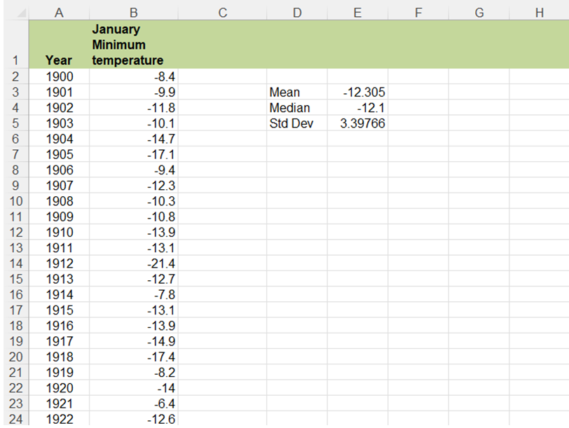
Fig. 1 The Excel file.
Create Histogram
- In a normal distribution, the mean, median, and mode are identical.
- Create a histogram of the temperature data.
- A histogram can be produced using the Data Analysis tool on the Data tab.
- Select Data Analysis and then Histogram. Fill in the pop-up window in the manner in Fig. 2 below:
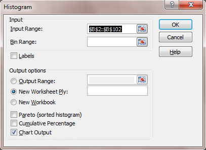
Fig. 2 The Histogram settings.
- Select Data Analysis and then Histogram. Fill in the pop-up window in the manner in Fig. 2 below:
- A histogram can be produced using the Data Analysis tool on the Data tab.
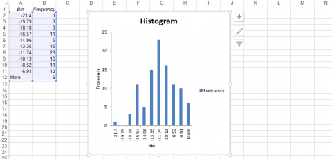
Finished Histogram
- The histogram is given below (Fig. 3):
Probability Plot
- We will now generate a normal probability plot
- Go back to the sheet with the data set and select Data / Data Analysis / Rank and Percentile.
- Fill in the pop-up window in the manner below (Fig. 4):
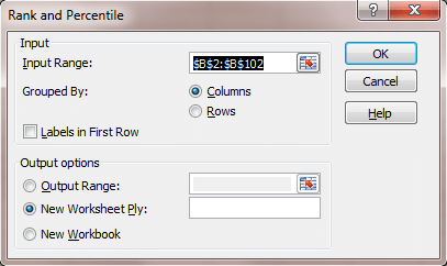
Fig. 4 Rank and Percentile dialog box.
- Fill in the pop-up window in the manner below (Fig. 4):
- Go back to the sheet with the data set and select Data / Data Analysis / Rank and Percentile.
Create Probability Plot
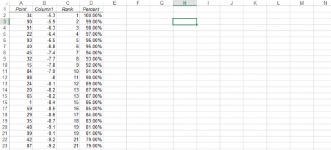
- On the page with the rank and percentile data, click on a cell to the right of Column D (Fig. 5). Select the Insert Tab and Scatter, then select the first type of scatter plot.
Finished Probability Plot
- When the plot window opens and is selected, the chart tools will be available. Click Select Data and Add under Legend Entries (Series).
- The X-values are the Percent column, and the Y-values are in Column 1. Do not select the column headings in the x or y ranges, as that will cause you to create a plot that is the inverse of what you should have.
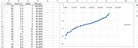
- Select OK twice, and the following plot will be visible (Fig. 6).
Evaluating the Distribution
Normally distributed data will fall along a straight line.
- A true Normal distribution is rare in a data set. It is up to the researcher to determine if the data are close to normally distributed. One informal test is to place a pen over the line of the Normal Probability Plot, and if there are few observations that can be seen then the observations are approximately normally distributed. There are also tests of Normality that can be used, but are not covered here.
- If the tails are above and below the straight line (as in this case), there is a little more variance than you might expect from a perfect normal distribution. If the tails are below the straight line, then the variance is less than expected from a normal distribution.
- This data are approximately normally distributed. While there are a few possible outliers, the normal probability plot and histogram suggest approximate normality.
Ex. 2: Calculate the Z-Statistic
Using Excel Formulas
Excel has built-in functions that calculate different parts of a normal distribution. Let’s examine how often monthly average minimum temperatures are expected to be below -17.78 in January.
There are many ways to find the answer to this question, and here we illustrate two. In the following, we are using the mean = -12.305 and standard deviation = 3.398 found for the normal curve in exercise 1.
One way to answer the question is to calculate the z-value for a temperature of zero.
Calculate z for the temperature = -17.78. z = (-12.305 – (-17.78))/3.398, or z = -1.61. The probability of a value less than this is 1 – 0.9463, where 0.9463 is the table value for z = 1.61. Our answer is 0.0537.
A second way to calculate this probability is to use Excel.
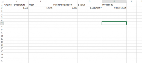
- Open a new Excel workbook (Fig. 7).
- Label the first column Original Temperature, the second Mean, the third Standard Deviation, a fourth column Z-Value, and the fifth column Probability.
- Enter -17.78 in the first row under temperature, -12.305 under the mean, and 3.398 under standard deviation.
- Enter the formula “=(A2 – B2)/C2” into the first row under z-value.
- Finally, enter the formula “=norm.s.dist(D2, TRUE)” in the cell below Probability.
Further Application
As you can see, the probability of a value being below any z-value can be computed with this formula.
- How often does a temperature of -17.78°C occur? According to these data, about once every 20 years.
- Try the same for the extreme value of -21.4. You should see that it is extremely unlikely for this low a temperature to occur. This would imply that the average low temperature for the entire month is -21.4°C, an extremely cold month!
- Calculate this by entering -21.4 into the second cell under Temperature, then copy and paste the mean, standard deviation, and two formulas into the rows next to the new temperature.
- To find the probability of a value falling between two values we have to do the calculation twice.
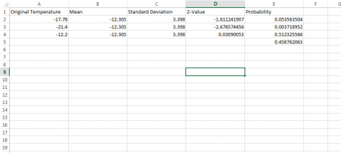
- Try this for values between -17.78 and -12.2°C.
- We already have the probability of temperatures less than 0 in the first row.
- Get the probability for -12.2 in another row. Since these are just probabilities of values less than these temperatures or z-values, we can subtract to get the probabilities of being between these two limits, 0.510-0.054 = 0.456.
- Thus, there is a 45.6% probability of average January minimum temperatures between -17.78 and -12.2°C (Fig. 8).
Confidence Interval for a Mean
Computing a Confidence Interval
For a normal population with known Standard Deviation δ, we can sample and compute a Confidence Interval for the Population Mean μ.
Suppose we want to estimate the true yield difference for 2 corn hybrids. From data comparing many pairs of corn hybrids, we know that the differences are normally distributed, and we also have very good knowledge of the standard deviation of these differences. We have a sample of 16 locations where the 2 corn hybrids are both planted and take the difference in hybrid yields. Each difference is an individual from a population of all such differences. A 95% confidence interval for the true average difference in hybrid yields is centered on the average difference ([latex]\bar{X}[/latex]) plus and minus 2 standard errors of the mean (σ/√n).
Estimating a True Mean
We use properties of the normal distribution and sample averages to get this confidence interval. The reasoning is as follows.
Suppose we have a normal distribution with known standard deviation σ, but the true mean µ is not known, and we wish to estimate it.
- We know from the properties of the normal distribution that 95% of the individuals differ from the true population mean by no more than 1.96 (about 2) standard deviations.
- By the central limit theorem, 95% of sample averages will differ from the population mean by less than about two standard errors (σ/√n).
- Therefore, we can estimate µ using the sample average,
 , and an interval of 1.96 σ/√n above and below it.
 - We have 95% confidence that this procedure will give correct results, provided our assumptions are met.
Null Hypothesis
Testing a Hypothesis
Designing an experiment to test a hypothesis begins with a statement that can be falsified with experimental data, i.e., the Null Hypothesis.
In the previous chapter, we used our knowledge of the normal distribution to examine how the high temperature in June of one year compared to the historical high temperature for that month. We wanted to know if the average high of 29.8°C differed from the historical mean of 27.6°C. To do this we calculated a z-value to determine how many standard deviations the observed value was from the historical mean. It is possible, however, to approach this question in another way. We could ask “is the high temperature observed for June of this year significantly different from the historical mean high temperature in June?” Using our knowledge of the normal distribution we can perform a statistical test to answer this question.
By convention, a statement stating no differences (null) is usually called a null hypothesis. In our example, the null hypothesis is that the observed high temperature is equal to the historical mean high temperature. This may be written symbolically as: H0:μ = μ0. The alternative hypothesis is that the means are not equal, or Hα:μ ≠ μ0. Ultimately our experimental data will either reject the null hypothesis or support it.
Errors Can Occur If the Null Is True or False
There are two types of errors that can occur when testing a null hypothesis (Table 1). The first type (I) is rejecting the null hypothesis when it is actually correct. The second type (II) is the opposite case; supporting the null hypothesis when it is incorrect. The probability of making a Type I error is called the significance level, denoted by the Greek letter alpha (α). A commonly used alpha level in agronomic experiments is 5%. This means that in one out of twenty tests a significant difference will be found where none actually exists. The probability of a Type II error is referred to as beta (ß) or the error of accepting the null hypothesis when it is not true. The errors are related; reducing the value of alpha increases the possibility of committing a Type II error. Choice of levels of alpha and beta depends on where you wish to assign the chance of error. In agronomic experiments, we are generally more concerned with controlling Type I errors than Type II errors because we consider the consequences of making a Type I error (saying there is a difference when there really is none) to be more serious. We will revisit this topic throughout the course.
| H0 is true | H0 is false | |
|---|---|---|
| H0 rejected | Type I | none |
| H0 not rejected | None | Type II |
Examining the Hypothesis
Returning to our example, we now need to determine the level of significance for our test. Since the consequences of our being wrong are not very great, let’s use an alpha level of 20%. This means that we will declare any temperature value that occurs less than 20% of the time based upon the normal probability distribution to be different from the historical mean. The alternative hypothesis here is that the June high temperature differs from the mean high temperature. It could be above or below the true mean. This is called a “two-tailed” test because we reject H0 if the June high temperature is either above or below the mean, i.e., in either the upper tail or lower tail of the distribution.
Now, let us assume that we have a normal distribution of monthly high temperatures with a known standard deviation (1.6°C). We want to find z-values for which 20% of the observations will be in the tails. We need 10% in each tail. Using a table of z-values with P = 10% in one tail, we find z = 1.2816. Since our calculated z-value 1.05 is less than 1.2816 we fail to reject the null hypothesis and conclude that the observed June high is not significantly different from the historical mean.
Study Question 5: Null Hypothesis
Here are the details on the two fields the farmer wishes to use. For simplicity, we assume each field has one soil type only (Table 2).
| Soil characteristics | Amount of organic matter and minerals |
| Field 1 16 hectares | |
| Sharpsburg – silty clay loam | moderate organic matter |
| 9-14% slope | low subsoil P |
| moderately well drained | medium subsoil K |
| surface layer depth is 8-18cm | n/a |
| subsoil layer depth is 122cm | n/a |
| Field 2 16 hectares | |
|---|---|
| Macksburg – silty clay loam | high organic matter |
| 0-2% slope | low subsoil P |
| somewhat poorly drained | medium subsoil K |
| surface layer depth is 61cm | n/a |
| subsoil layer depth is 140cm | n/a |
Option 1
The farmer decides to plant Field 1 with the new variety and Field 2 with the old variety. When he harvests, he finds the following results (Table 3):
| Field 1 | Field 2 |
|---|---|
| New yield variety: 8780 kg/ha | Old yield variety: 9410 kg/ha |
Option 2
The farmer decides to plant Field 1 with the old variety and Field 2 with the new variety. When he harvests he finds the following results (Table 4):
| Field 1 | Field 2 |
|---|---|
| Old yield variety: 7530 kg/ha | New yield variety: 10660 kg/ha |
Option 3
Realizing that there is a soil fertility difference between the fields, he decides the plant half of each field with each variety. This produces the following results (Table 5):
| Field 1 – Plot 1 | Field 1 – Plot 2 | Field 2 – Plot 1 | Field 2 – Plot 2 |
|---|---|---|---|
| Old yield variety: 7530 kg/ha | New yield variety: 8780 kg/ha | Old yield variety: 9410 kg/ha | New yield variety: 10660 kg/ha |
Experiment Conclusions
Usually, it is difficult to limit both Type I and Type II errors. The decision must be made on which error is least detrimental in the decision-making process. This usually includes economic factors in the decision-making. You can limit both errors by increasing the number of units in a sample.
What Does It Mean To “Accept The Null Hypothesis?”
It only means that our data do not provide enough evidence to reject the null. It doesn’t mean that the null hypothesis is definitely true. For example, two people form null hypotheses; person A says his null is that the true corn yield difference is zero, person B says the true difference is 0.1. An experiment is run, and we fail to reject the hypothesis of A. Does this mean he is right and B is wrong? Of course not. The difference might be small and just not detected in the experiment.
The null hypothesis is a “straw man” set up to be torn down by experimental evidence. We may just not have enough evidence to reject H0. So we fail to reject H0 even though it may not be the true state of nature. If you see the words “accept the null hypothesis“, you should mentally translate to “fail to reject the null hypothesis“.
Testing a Hypothesis
Soil Sampling Example 1
Let’s take a different example, fertilizer recommendations. Return to our soil sampling example (below) from Chapter 2 on Distributions and Probability. You are sampling here to determine if potassium fertilizer is necessary. ISU recommendations are for soil K to be between 70 and 130 ppm. Usually, you are checking to see if there is sufficient K. You decide to apply fertilizer if the soil K is less than 130 ppm. Your hypothesis here is:
H0: sampled soil potassium is greater than or equal to 130 ppm (no action is taken)
Hα: sampled soil potassium is less than 130 ppm (fertilizer must be applied)
This is chosen because your action to be taken is to apply fertilizer. You want to be assured that you need fertilizer before applying. Economically, though, K is not very expensive to apply. So, your criterion for significance is not very high. You are willing to risk a larger chance of a Type I error for a smaller Type II error. You are more willing to reject your null hypothesis when it is true (to apply fertilizer when none is needed) than to accept your null hypothesis when it is false (to not apply K even though it is needed).
Soil Sampling Example 2
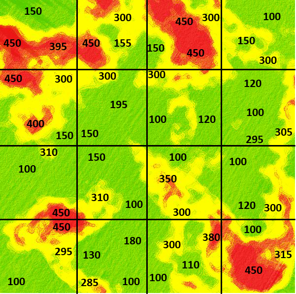
Click on the field to sample that location (square) (Fig, 9). Select sets of locations to calculate an average potassium value for the field. For example, a set with 300, 150, and 450 would result in a mean of 300.
What does this suggest about how to design a sampling scheme to best represent the “population” mean value for the field? What happens when you increase the number of samples or vary their location? Would it be better to be random in your sampling scheme or systematic?
If you do this computation several times, pressing the Reset button between sets, you will notice that variation in the calculated average value occurs depending on where the samples are drawn.
Sampling Exercise Application
What does this suggest about how to design a sampling scheme to best represent the “population” mean value for the field? What happens when you increase the number of samples or vary their location? Would it be better to be random in your sampling scheme or systematic?
If you do this computation several times, you will notice that variation in the calculated average value occurs depending on where the samples are drawn.
We see from this activity that it is difficult to get a representative sample for measuring an underlying parameter of the population, such as the average potassium concentration in an entire field. Taking three observations, and calculating a mean from them, better represents the true population mean than would an individual value. More than three observations would be even better.
It is generally better to take a random sample than a systematic one. Random samples provide a method to get unbiased estimates of population values. W.G. Cochran gives an example illustrating this on page 121 of his book Experimental Designs, co-authored with Gertrude Cox. Even experts have a bias when trying to select a representative sample.
In an experiment to measure the heights of wheat plants in England, several expert samplers chose what they thought were eight representative plants from each of six small areas containing about 80 plants. Every expert ended up choosing samples taller than the average of all the plants in the area. Of the 36 total samples, only 3 had shorter average wheat height than the corresponding area. Samplers averaged from 1.2 cm to nearly 7 cm over the actual height for systematic samples compared with the actual average for the six plots. It is likely that their eyes were drawn to the taller plants. A properly conducted random sampling scheme would have avoided this bias.
Sampling Conclusions
Think about the samples you gathered when sampling the soil potassium situation in this example. What values did you get? The actual average of the field is somewhere near 225 ppm. However, at this point we do not know the variability in the samples to test for significance. If we had knowledge of the distribution and the true variances of soil K measurements in the field, we could use the normal distribution and test the hypothesis. But at this stage, we cannot test the value specifically because we do not know whether we have a normal distribution with known standard deviation. We will discuss that more in a later unit.
Hypothesis Testing
Normal Distribution And Hypothesis Testing
Decisions on varieties to plant or whether to apply fertilizers are made many times by producers. They do not realize they are using a scientific method to make the decision, though. The actual method of making the decision proceeds using the steps below:
- Clearly decide the population and set a definable null and alternative hypothesis.
- Choose a significance level at which you are comfortable, i.e., where the possibility of random error will not cause you to make a poor choice. If you are reasonably comfortable that Type I error of 5% is acceptable, use it. If you wish to be more certain not to wrongly reject your null hypothesis, choose a smaller alpha. Be aware that doing this opens the door for accepting the null hypothesis when it is not true (Type II error).
- Compute the statistic to be tested. How does the statistic compare with what you expect for the population if the null hypothesis is true?
- Use the calculated statistic to accept or reject your null hypothesis.
When the population follows a normal distribution with known variance, you can test the hypothesis as in the June temperature example. If you are sampling from an approximately normal distribution, with unknown variance, then we will need to use a t-statistic, which is the subject of a later unit.
Summary
Sample averages
- From a normal distribution are also normally distributed.
- Have variance estimated by [latex]\dfrac{{S^2}}{n}[/latex].
- Variance of sample means is reduced by factor [latex]\dfrac{1}{n}[/latex].
Central Limit Theorem
- Even sample means from non-normal populations become normally distributed as n gets large.
- This allows us to make probability statements (confidence intervals).
Confidence Intervals
- A [latex]95\%[/latex] CI for [latex]\mu[/latex] is [latex]Y\pm{1.96}\dfrac{\sigma}{\sqrt{n}}[/latex].
- A [latex]99\%[/latex] CI for [latex]\mu[/latex] is [latex]Y\pm{2.58}\dfrac{\sigma}{\sqrt{n}}[/latex].
Hypothesis Tests
- Start with null hypothesis (no treatment effect).
- Type I errors when true null is rejected.
- Type II errors when false null is accepted.
- Based on probability, we reject or we fail to reject H0, and then draw conclusions.
The Chapter Reflection appears as the last “task” in each chapter. The purpose of the Reflection is to enhance your learning and information retention. The questions are designed to help you reflect on the chapter and obtain instructor feedback on your learning. Submit your answers to the following questions to your instructor.
- In your own words, write a short summary (< 150 words) for this chapter.
- What is the most valuable concept that you learned from the chapter? Why is this concept valuable to you?
- What concepts in the chapter are still unclear/the least clear to you?
How to cite this chapter: Mowers, R, D. Todey, K. Meade, W. Beavis, L. Merrick, A. A. Mahama, & W. Suza. 2023. Central Limit Theorem, Confidence Intervals, and Hypothesis Tests. In W. P. Suza, & K. R. Lamkey (Eds.), Quantitative Methods. Iowa State University Digital Press.
definition
This is the question that is trying to be proven incorrect. Usually, this occurs when trying to prove some treatment causes a significant difference from expected. Opposite of alternative hypothesis.
the opposite of the null hypothesis. This is what is usually wanted to be proven true.
