
Chapter 6: Continuous Data
Ron Mowers; Ken Moore; M. L. Harbur; Kendra Meade; William Beavis; Laura Merrick; Anthony Assibi Mahama; and Walter Suza
In this chapter, we will learn that sample means from a population that has a Normal distribution are also distributed as Normal, but with a smaller variance that has a population. We will then extend the concept to samples from two populations. For example, sometimes, we want to identify the best management practice between two alternatives. Such as comparing the use of starter fertilizer to no starter fertilizer, or one corn hybrid against another, or a new insecticide against a common one. In all of these comparisons, the key question to be answered is, “Are the means of the populations representing the two treatments the same.” In the language of statistics, this is called a two-sample hypothesis; the most common method for testing it is the t-test.
- How the distribution of a set of sample means around their population mean can be described in terms of t-values
- How to calculate the t-value for sample means as related to their population means
- How a confidence limit describes a range of possible values for the population mean, μ
- How a t-test can be used to determine whether the difference between two sample means is significant
- How to conduct t-tests using Excel
The t-Distribution
The t-distribution is used for sample mean when the variance is not known. Statistical standards must apply to a wide variety of research, from corn yield trials to soybean disease studies to nitrate sampling in groundwater. Even within one of these categories, the amount of variability may differ from one month or year to the next. Therefore, we need to describe the distribution of our sample means according to the distribution curve itself, and in a way that is unitless. We cannot use the normal distribution described in Chapter 2 on Distributions and Probability because we do not know the variance. We define this distribution of sample means in terms of the t-distribution.
As we learned, the shape of the distribution curve for sample means is based on the number of observations per sample. Our values for t will also vary with the number of observations or replications, that occur. However, for normally distributed variables and a given number of degrees of freedom (df), we know that 95% of the sample means will lie within a particular t-value of the mean. This t-value remains the same, for the given df, whether we are studying swine, alfalfa, or soil moisture.
What are degrees of freedom? In general, the number of degrees of freedom associated with a set of sample means is the number of individuals in the sample used to calculate the mean minus 1.
A Sample t-Value Table
For example, look at the following t-value table. For a sample size of 5, 95% of the sample means will be within plus or minus 2.776 standard errors (S/√n) of the mean:
| Degrees of Freedom | Percentage Points in Top Tail | ||||
|---|---|---|---|---|---|
| 5 | 2.5 | 1 | 0.5 | 1 | |
| 1 | 6.314 | 12.706 | 31.821 | 63.657 | 318.309 |
| 2 | 2.920 | 4.303 | 6.965 | 9.925 | 22.327 |
| 3 | 2.353 | 3.182 | 4.541 | 5.841 | 10.215 |
| 4 | 2.132 | 2.776 | 3.747 | 4.604 | 7.173 |
| 5 | 2.015 | 2.571 | 3.365 | 4.032 | 5.893 |
| 6 | 1.943 | 2.447 | 3.143 | 3.707 | 5.208 |
| 7 | 1.895 | 2.365 | 2.998 | 3.499 | 4.785 |
| 8 | 1.860 | 2.306 | 2.896 | 3.355 | 4.501 |
| 9 | 1.833 | 2.262 | 2.821 | 3.250 | 4.297 |
| 10 | 1.812 | 2.228 | 2.764 | 3.169 | 4.144 |
| 11 | 1.796 | 2.201 | 2.718 | 3.106 | 4.025 |
| 12 | 1.782 | 2.179 | 2.681 | 3.055 | 3.930 |
| 13 | 1.771 | 2.160 | 2.650 | 3.012 | 3.852 |
| 14 | 1.761 | 2.145 | 2.624 | 2.977 | 3.787 |
| 15 | 1.753 | 2.131 | 2.602 | 2.947 | 3.733 |
In this example, a sample with four degrees of freedom will have 5% of the distribution 2.776 × t above the mean and another 5% of the distribution 2.776 × t below the mean.
Sample Means in Values of t
Now that we understand how t values relate to the distribution curve for a set of sample means, we must learn how to express our sample means in values of t. This is given by the following formula:
[latex]t=\frac{\hat{Y}-{\mu}}{S_{\hat{y}}}[/latex]
[latex]\text{Equation 1}[/latex] Formula for computing t value,
where:
[latex]\hat{Y}[/latex] = sample mean,
[latex]\mu[/latex] = population mean,
[latex]S_{\hat{y}}[/latex] = standard error of the sample mean = [latex]\frac{S}{\sqrt{n}}[/latex].
We use the t-value rather than z because we are estimating σ2 with s2. The t-value represents the difference between a particular sample mean and the mean of the whole population of sample means as a function of the standard error for that population, Sy = S/√n. Stated more simply, the t-value is the number of standard errors a particular sample mean is from the average value for all of the sample means. This tells us whether our difference is large in relation to the variation of our sample.
t-Value Scenarios
For example, a 500 kg/ha difference between the sample mean of a certain corn hybrid and the population mean of all corn hybrids would not be a large difference when we are dealing with corn (which might have a standard error of 750 kg/ha for a given number of plots) as when we are studying soybean (which could have a standard error of 250 kg/ha for the same number of plots). The t-values for each of these scenarios are given below:
Corn:
[latex]t=\frac{\hat{Y}-{\mu}}{S_{\hat{y}}}=\frac{250kg}{750kg}=0.34[/latex]
[latex]\text{Equation 2}[/latex] Corn example of t value computation,
Soybean:
[latex]t=\frac{\hat{Y}-{\mu}}{S_{\hat{y}}}=\frac{500kg}{250kg}=2.00[/latex]
[latex]\text{Equation 3 Soybean example of t value computation}[/latex]
Confidence Limits & Intervals
Confidence intervals (CI) are used to describe a range of values for a set of sample means from multiple samples of the same population. A CI does not predict that the true population mean will be included in the interval.
We can set the ranges for our confidence interval using Excel. You will learn how to do this in the Excel lab for this chapter.
We use the term confidence to remind us that the variation associated with this procedure is the result of our own experimental and sampling techniques. Stated otherwise, the population mean in which we are interested stays the same — it is our confidence interval that shifts according to the number of and particular samples in our set. There is no probability or chance associated with the population mean but rather with the value of the sample means.
Ex. 1: Calculating a Confidence Interval
Often we are asked to make decisions about some characteristic of a population based on samples selected from it. In this example, we will consider the protein value of two lots of alfalfa hay.
The data in the Alfalfa Quality worksheet were collected from two lots of hay that were offered for sale at auction. Each lot was first-cutting hay and weighed approximately 30 tons. Based upon a one percentage unit difference in the protein analysis, lot 2 was discounted $10 per ton because the buyer claimed it was less than 15.5% protein. The buyer’s method to see if a lot is less than 15.5% is to calculate a 95% confidence interval for protein and see if it includes 15.5%.
Our first question should be, “How confident are we that the sample means represent the true mean.” One approach to answering this question is to calculate a confidence interval for the mean of each sample population.
STEPS
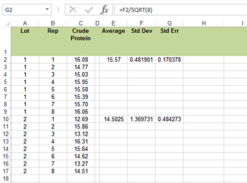
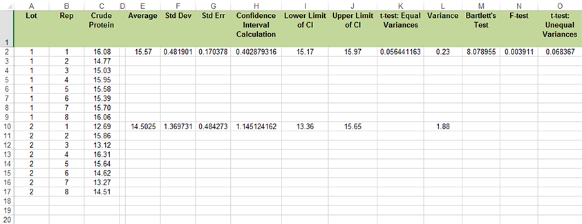
- Calculate the 95% confidence interval of the sample mean for each lot. Download and open the Excel file QM-mod6-ex1data.xls.
- There should be three columns: Lot, Rep, and Crude Protein.
- We will calculate a mean, standard deviation, and standard error for each lot. Use the Average and STDEV.S to calculate the mean and standard deviation of each lot sample. Then use the standard deviation to calculate the standard error by dividing the standard deviation by the square root of the number of samples in a lot (Fig. 1).
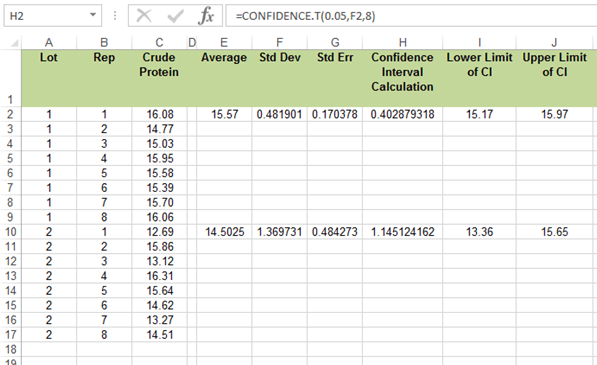
It is possible to use Excel to calculate a confidence interval from a t-distribution using the formula Confidence.T. The arguments are the alpha level, standard deviation, and the number of samples or replications.
- Now subtract and add the calculated value from the mean to find the confidence interval.
- Now, we will hand calculate the confidence interval to see that it matches that given by Excel. Use Equation 4 and the SE from Excel. Use the t-value for 5% probability in two tails (2.5% in one tail) from either Appendix 3 or the t-table given earlier in this unit. Remember, there are 7 df for 8 reps in each sample.
- Calculate the 95% confidence interval for each lot (Fig. 2).
- Do the two confidence intervals overlap?
- Save the file to your desktop for use in the next exercises.
Discussion
Should Lot 2 have been discounted for a small difference? Support your assertions.
t-Tests For Significance
t-tests can be used to compare two treatment means.
Confidence intervals may work well for single samples compared to the mean. But what can we use to compare the two samples? We can also use t-values to determine whether the calculated mean values of two sample sets are significantly different. This difference can be expressed in terms of t:
[latex]t=\frac{\bar{d}-{\mu_{\bar{d}}}}{S_{\bar{d}}}[/latex]
[latex]\text{Equation 4}[/latex] Formula for computing t value to compare two treatment means,
where:
[latex]\bar{d}[/latex] = difference between sample means,
[latex]\mu_{\bar{d}}[/latex] = difference between population means,
[latex]S_{\bar{d}}[/latex] = standard error of the difference.
In most cases, we are trying to identify any significant difference; the value we use for the mean difference is zero. A zero value for a mean difference, therefore, represents the null hypothesis that there is no treatment effect. Our t-value expresses the actual difference between the two sample means as a function of the standard error of the difference. Again, it is this conversion that makes the difference meaningful regardless of what particular variable we are measuring.
Paired t-Test
It is at this point that we must know more about the experiment or how the populations were sampled in order to compute Sd. If both treatments of an experiment are applied to units that are paired in blocks, we use a paired t-test method. If the populations are independent or treatments are applied completely at random to the experimental units, we use what is called an independent samples t-test. Each of these has a different standard error of the difference Sd.
Suppose first that the treatments are on units that are naturally paired (and thus not independent). An example is a test for differences in two wheat varieties, each grown in the same block or area in a field for 5 different blocks. There is a natural pairing of the varieties because they each appear in each block even though they have been randomly assigned to either the left or right side of the block. Another example is a test of side dressing of nitrogen fertilizer vs the check of no additional fertilizer, each applied to half a field on fields from 12 different farms.
For the paired t-test, the computation of the t-value is easy. Just take the differences of treatment 1 – treatment 2 for each pair. Then, use these differences as the data and compute the t value as done in equation 1. The d in equation 5 is just the average of the differences, and the Sd is the square root of Sd2/n. The variance of the differences is Sd2, and number of pairs is n. The test of the null hypothesis that treatments have the same mean is just a test of differences being zero, H0: μd = 0. We will see in the Excel exercises how this is done.
Independent Samples t-Test
The independent samples t-test, done for independent populations or samples, uses the Sd given in Equation 5 below. One independent sample example is a set of 24 pots of soybeans in a growth chamber, half of which receive a zinc foliar supplement, while the other half receive no supplement. The pots which receive the treatment are randomly chosen, for example, pots 2, 3, 7, 9, 10, 11, 13, 14, 16, 18, 21, and 24. Sometimes samples are considered to be independent when they are drawn at random from two mutually-exclusive populations, for example, a poll on farmers’ opinions on a land-use policy, with 100 respondents in Illinois having an average farm size of over 1000 acres and another 100 with farms less than 1000 acres. It is important that these samples be chosen at random for a valid comparison.
When populations are independent, as in the 2-sample case, the variance of a difference is the sum of the two variances. In the 2-sample (independent samples) case, the variance of a difference in sample means [latex](\bar{x}_1+\bar{x}_2)[/latex] is the sum of their variances [latex](S^2_\bar{x_1}+S^2_\bar{x_2})[/latex], where subscripts indicate the population. In equation 5, the standard error used to divide the mean difference is the square root of the sum of the variances associated with x1 and x2:
[latex]S_{\bar{d}}=\sqrt{S^2_{1}+S^2_{2}}[/latex].
[latex]\text{Equation 5}[/latex] Formula for computing the standard error of the difference between two treatment means,
where:
[latex]S_{\bar{d}}[/latex] = standard error of the difference between sample means,
[latex]{S^2_{1}}[/latex] = variance from sample population [latex]{x}{_1}[/latex],
[latex]{S^2_{2}}[/latex] = variance from sample population [latex]{x}{_2}[/latex].
Calculation Results
In many texts, the standard error of the difference is calculated as:
[latex]S_{\bar{d}}=\sqrt{\dfrac{S^2_{1}}{n_1} + {\dfrac{S^2_{2}}{n_2}}}[/latex]
[latex]\text{Equation 6}[/latex] Formula for computing standard error of the difference,
where:
[latex]S_{\bar{d}}[/latex] = standard error of the difference between sample means,
[latex]{S^2_{1}}[/latex] = variance from sample population [latex]{x}{_1}[/latex],
[latex]{S^2_{2}}[/latex] = variance from sample population [latex]{x}{_2}[/latex]
[latex]{n_{1}}[/latex] = sample size for population [latex]{1}[/latex],
[latex]{n_{2}}[/latex] = sample size for population [latex]{2}[/latex].
This is because the variance of population 1 is calculated as:
[latex]{S^2_{1}} = \dfrac{S^2_{1}}{n_1}[/latex].
[latex]\text{Equation 7}[/latex] Formula for computing the variance for population 1,
and likewise for population 2.
Since both samples have variability involved, both variables must be accounted for. The number of degrees of freedom associated with this difference is either calculated by the computer, or if done by hand, is the degrees of freedom associated with the smaller sample. For samples of equal size, and if we can assume S12 = S22, the number of degrees of freedom is 2(n-1).
After calculating the t-value of the difference in which we are interested, we then look up the critical table t-value, for which there is only a 5% chance of a larger value occurring. Generally, we have critical t-values of about 2, or slightly higher, for a 0.05-level two-tail test. If the t-value of our difference exceeds the critical t-value, then we say that we have a significant difference between the two means. Would a significant t-test indicate that the two populations are truly different?
There are three classes of t-tests that are commonly used in agronomic experiments (which can be calculated using Excel:
Ex. 2: t–test assuming equal variances
There is a more direct approach to comparing the means of two sample populations – the t-test. In our alfalfa example, suppose the populations have equal variances, and what we really want to know is whether or not the two sample means are different from one another. This question can be stated as a simple statistical hypothesis: H0:μ1=μ2 vs. the alternative Ha: μ1 ≠ μ2. In this exercise, we will use the t-test procedure in Excel to test this hypothesis.
Exercise 2
- Perform a t-test to compare mean protein concentrations of the two alfalfa lots using the following steps (Fig. 3): Open the file created in QM-mod6-ex1data.xls.
- Label a new column, ‘t-test: Equal variance,’ and in the first row under the title, enter the formula “=T.TEST(C2:C9,C10:C17,2,2)”.
This dictates that the observations for the first sample are in C2:C9, the second set are in C10:C17, it is a two-tailed test, and that this is an independent sample t-test assuming equal variances.
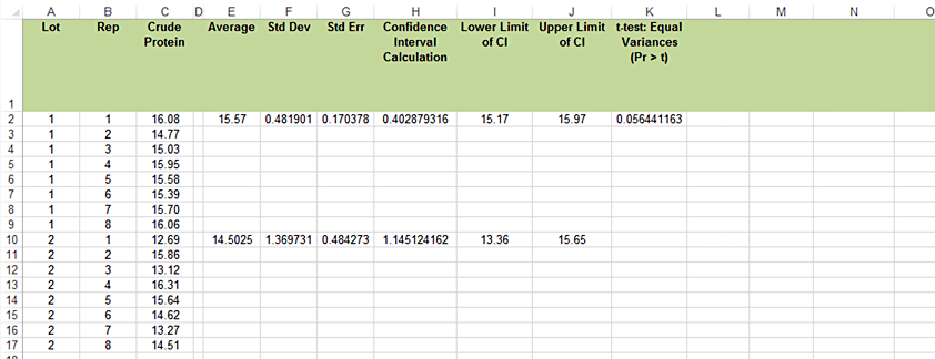
- Read the results of the t-test (assuming equal variances) as Prob > |t|. This is the probability, assuming the null hypothesis is true, of observing the results in your data set, and is 0.0564.
- Note that the t-test is assuming equal variances and has a two-tailed alternative. To convert the probability to a one-tailed alternative, divide the two-tailed probability by 2. It is 0.0564/2 = 0.0282.
- Do the means differ? (Is the Lot 1 mean significantly lower than the Lot 2 mean based on these samples?)
Ex. 3: t-Test Assuming Unequal Variances
You may have noticed in the t-test output from the last exercise that the standard error for Lot 2 is about three times as great as that for Lot 1.
One of the assumptions we made for the t-test was that the two sample populations shared a common variance. Hence, a pooled estimate of the population variance was used in the test.
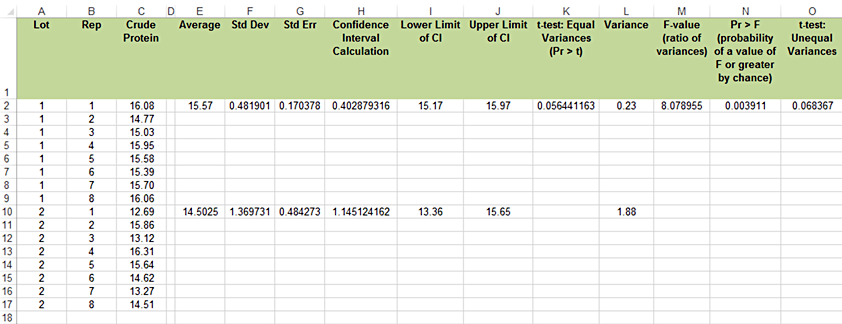
We can easily test the hypothesis that the two variances are equal by computing a simple F test (Fig. 4):
- Open the QM-mod6-ex1data.xls file.
- Calculate the variance for each lot in a new column using the formula Var.S.
- Divide the larger of the two variances by the smaller one to calculate F.
- Determine the critical F value. (Numerator and denominator df are those from the two samples.) The alpha level is 0.05.
- If the calculated F is greater than the critical F, we conclude that the variances are different and use another t-test.
- If the calculated F is less than the critical F, we conclude that the variances are the same and that a pooled variance was appropriate for the t-test.

For our example, the calculated F is (1.88/.23) = 8.17 and the critical F = 3.79. Therefore, we conclude that the variances of the two sample populations are different and a different t-test is required (Fig. 5).
- It is possible to find a p-value for this test using “=F.DIST.RT(M2,8,8)”. M2 is the cell with the F-ratio in it.
Note, however, that this test and other tests for equality of variance are not robust procedures. We saw earlier that the t-test is reasonably robust. It returns fairly accurate probability statements for samples from similarly shaped distributions when sample sizes are nearly equal. The F-test for variances, however, is very sensitive to non-normal distributions.
Exercise 3
Perform a t-test to compare mean protein concentrations of the two alfalfa lots. This is the same hypothesis as Exercise 2: H0:μ1 = μ2 vs. the alternative Hα: μ1 ≠ μ2 Use the following steps:
- Label a new column ‘t-test: Unequal Variances’ (Fig. 6).
- This time, we again look for the P>|t| for the test of the null hypothesis that the means for the two lots are equal.
- Use the same formula from Exercise 2, but dictate that the required test assumes unequal variances.
- For the test with unequal variance, P = 0.0684. This is again for the two-tailed alternative, by default.
Ex. 4: Paired t-test
Sometimes data collected from two sample populations are related in some way. When this occurs we say that the observations are paired. A good example of this is the strip design that is often used in on-farm trials to compare two treatments. Treatments are applied to strips that run across a field in such a way that every adjacent pair of strips contains both treatments. Treatments are randomly allotted to strips within each pair. For a more complete description of this methodology read the paper by Exner and Thompson.
Exercise 4
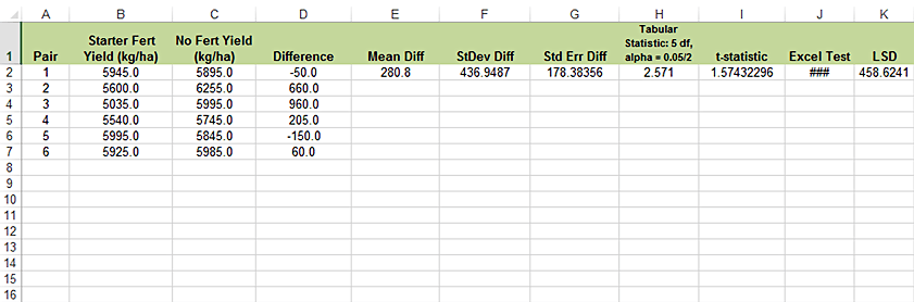
- Perform a paired t-test to determine if starter fertilizer had an effect on corn yield using the following steps:
- Download and open the Excel file QM-mod6-ex4data.xls.
- We will first calculate the paired t-test step-by-step (Fig. 7).
- Calculate the difference between each pair of observations.
- Calculate the mean of the differences.
- Now calculate the standard deviation, using Stdev.S.
- The standard error is the standard deviation divided by the square root of the number of pairs.
- The t-statistic is the mean divided by the standard error.
- The calculated value is less than the tabular value, so we fail to reject the null. There is not a significant difference between the two treatments.
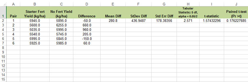
- Excel also contains a formula to calculate a paired t-test. It is essentially the same as the one used in Exercises 2 and 3: “=T.TEST(B2:B7,C2:C7,2,1)” (Fig. 8). However, the two arrays are the sets of observations from the two treatments sorted by pairs, and the last variable is one to indicate a paired test.
Did the use of starter fertilizer have any effect? No, since Prob > |t| = 0.18, we do not reject the null hypothesis and conclude there is no statistically significant effect.
Two-Sample Hypothesis Testing
There are three sets of hypotheses that can be tested with a t-test (Table 2).
| Set | Null Hypothesis | Alternative Hypothesis |
|---|---|---|
| 1 | [latex]\mu_{1}=\mu_{2}[/latex] | [latex]\mu_{1}\neq\mu_{2}[/latex] |
| 2 | [latex]\mu_{1}\ge\mu_{2}[/latex] | [latex]\mu_{1}\lt\mu_{2}[/latex] |
| 3 | [latex]\mu_{1}\le \mu_{2}[/latex] | [latex]\mu_{1}\gt\mu_{2}[/latex] |
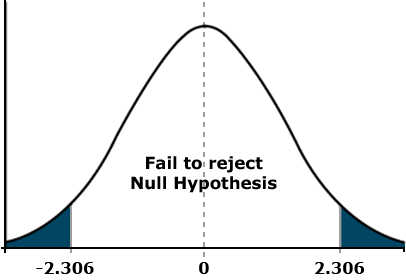
The first set simply states that there is either a difference between the two means or there is not. The alternative hypothesis gives no regard to how the two means may differ but simply states that they are different in some way. We use this hypothesis when we do not have a preconceived idea as to how the means will differ. For example, if we are comparing yields of two highly recommended varieties, we probably have no expectation of which will be greater. This type of comparison is called a two-tailed test because we want to know if the observed t lies within either tail of the distribution (Fig. 9). Assuming a mean difference for the two varieties of 250 kg/ha, a standard error of 120, and 8 df the test would look like this:
[latex]t=\frac{\bar{d}}{S_{\bar{d}}} = \frac{250}{120}=2.083\lt {\text{}t_{{0.05, 8df}} = 2.306}[/latex].
[latex]\text{Equation 8}[/latex] Example calculation of t for two-tailed test,
Test Conclusion
In this example, since our calculated t is less than the tabular t, we fail to reject the null hypothesis and conclude that the means are not significantly different at alpha 0.05.
Direction of the Mean Difference
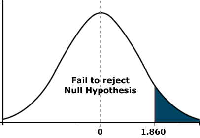
With the other two sets of hypotheses, we consider the nature or direction of the mean difference. For the alternative hypothesis, we want to know if the mean for population 1 is significantly smaller (set 2) or larger (set 3) than the mean of population 2. We use one of these hypotheses when we have an expectation about how the means will differ. For example, if we are comparing the yield of a new variety with that of an older control variety, we expect the new one to outperform the old one. This type of comparison is called a one-tailed test (Fig. 10) because we want to know if the observed t lies within one tail of the distribution. Assuming a mean difference for the two varieties of 250 kg/ha, a standard error of 120, and 8 df, the one-tailed test would look like this:
[latex]t=\frac{\bar{d}}{S_{\bar{d}}} = \frac{250}{120}=2.083\lt {\text{}t_{{0.05, 8df}} = 1.860}[/latex].
[latex]\text{Equation 9}[/latex] Example calculation of t for one-tailed test,
Calculate t Results
In this case, the calculated t exceeds the tabular t, and we conclude that the mean difference of 5 bu/acre is significant. The tabular t for a one-tailed test can be obtained from Appendix 3 in your text. However, the probability values listed in Table 1 are for a two-tailed test. To convert these values to probabilities for a one-tail test, divide them by 2. For our example above, you would use the t-values listed under 0.100 because 0.100 divided by 2 equals 0.05. The reason t-values differ for one and two-tailed tests has to do with the shaded areas of the curve. In the two-tailed test above, each shaded area represents 2.5% of the total area under the curve. For the one-tailed test, the shaded area under the right tail represents 5% of the total area.
Linear Additive Model
Underlying the two sample experiment is a linear additive model. Linear models are mathematical representations of the variables contributing to the value of an observation. The observed response is partitioned into effects due to treatments and the experimental units. That is, each measured response is an additive function of the treatment effect and a random effect error associated with the experimental unit on which the measurement was made.
The linear model for the t-test is:
[latex]Y_{ij}=\mu + T_{i} + \varepsilon_{(i)j}[/latex],
[latex]\text{Equation 10}[/latex] Linear model for t-test,
where:
[latex]S_{\bar{d}}[/latex] = standard error of the difference between sample means,
[latex]Y_{ij}[/latex] = response observed for the [latex]ij^{th}[/latex] experimental unit,
[latex]\mu[/latex] = overall population mean,
[latex]T_{i}[/latex] = effect of the [latex]i^{th}[/latex] treatment,
[latex]\varepsilon_{(i)j}[/latex] = effect associated with the [latex]ij^{th}[/latex] experimental unit; commonly referred to as error}.
Assumptions for Linear Models
Now let’s look at an example to see if we can make better sense of all this. A sales representative puts out a demonstration plot to compare a new herbicide product with an older one. Being a clever person, she has replicated each herbicide treatment four times. She, therefore, has eight plots and will have eight observations for each variable measured. The linear additive model Equation 11), for example, plot 3 of this experiment says the observed response (number of weeds) in the plot equals the overall mean response for the population plus an effect due to the herbicide applied plus a random effect due to the plot itself. This latter effect acknowledges that there will be some differences in the measured response among plots receiving the same herbicide treatment.
[latex]\text{Number of weeds in plot 3 = Average of all plots + Effect of Herbicide 2 + Plot 3 error}[/latex],
[latex]\text{Equation 11}[/latex] Linear additive response to herbicide in an individual plot,
Essential assumptions for linear models:
- Additivity – the effect of each term is additive.
- Treatment effects are constant for all experimental units (plots).
- The effects of plots are independent and not related to treatment effects.
The linear additive model for an experiment determines how the data are to be analyzed. We will revisit this topic in later lessons as we discuss the analysis of variance.
Confidence Limits
Least Significant Difference
The least significant difference (LSD) allows an easy test for the difference between two treatment means.
Earlier, we established confidence limits for our sample mean. The same procedure can be applied to a difference between two means, using the t-value of the difference between the two means. The confidence interval for the difference between two means is:
[latex]\text{CL}=\bar{d}\pm t_{S_{\bar{d}}}[/latex],
[latex]\text{Equation 12}[/latex] Formula for calculating CL,
where:
[latex]\bar{d}[/latex] = the difference between sample means,
[latex]{S_{\bar{d}}}[/latex] = standard error of the difference.
Confidence intervals (CI) for the true mean difference μd are obtained by computing the difference in means, d, and adding and subtracting t standard errors of d. To test the null hypothesis that μd is zero, we just see if zero is within the CL, and fail to reject the null if it is. This actually gives us an easy way to test the null hypothesis of zero difference: subtract the means and see if the difference is larger than tsd.
The least significant difference (LSD) between two sample means is simply this difference:
[latex]\text{LSD}=t_{S_{\bar{d}}}[/latex],
[latex]\text{Equation 13}[/latex] Formula for calculating LSD,
where:
[latex]{S_{\bar{d}}}[/latex] = the standard error of the difference,
[latex]t[/latex] = t-value for the appropriate df and probability.
Comparing Several Means
But what if we are comparing not one or two means but several? For example, what if we were comparing the grain yield of five corn varieties? We would then have to calculate the differences among all varieties (Table 3).
| Variety 1 vs. Variety 2 | Variety 1 vs. Variety 3 | Variety 1 vs. Variety 4 | Variety 1 vs. Variety 5 |
| Variety 2 vs. Variety 3 | Variety 2 vs. Variety 4 | Variety 2 vs. Variety 5 | n/a |
| Variety 3 vs. Variety 4 | Variety 3 vs. Variety 5 | n/a | n/a |
| Variety 4 vs. Variety 5 | n/a | n/a | n/a |
That is, ten different comparisons from a relatively simple experiment! Would it not be nice if we could know whether there were any significant differences to be found before we conducted this series of comparisons? As we will learn later, there is such a way.
Ex. 5: Determining the LSD
Having reached the conclusion that the 280 kg/ha difference between strips receiving starter fertilizer and those that did not was nonsignificant, you might be wondering just how large a mean difference it would take to be declared statistically different. We can answer this question easily by calculating the least significant difference (LSD).
The LSD is the smallest mean difference that can be declared significantly different from zero. Its value depends on the standard error of the mean difference (SED) and the number of degrees of freedom associated with it. The formula for calculating the LSD is [t x (SED)], where t is the tabular t for the error df at whatever level of significance is desired. In agronomic research, we often use the 0.05 probability level for this purpose.
Exercise 5
Calculate the LSD for the starter fertilizer experiment using the following steps (Fig. 11):
- From the Exercise 4 Excel workbook of moments for the differences (QM-mod6-ex4data.xls), find the standard error of mean difference (SED = 3.57).
- From the t-table, either at the start of this unit or in Appendix 3, find the tabular t for a two-tailed probability of 0.05. Remember, this is based on (6-1) = 5 df and the alpha level of 0.05 must be divided by two for a two-tailed test.
- Multiply the table t-value (2.571) and the SED to get the LSD = 9.18.
Summary
T-Distribution
- Used for sample means when variance is not known, but estimated.
- Depends on degrees of freedom (df).
- As df gets large, t-distribution becomes same as normal.
T-Values
- Like z-value, but used when we estimate variance.
- Tells how many standard errors from the mean.
Confidence Intervals (CI)
- Give range for the population mean μ.
- Interval is Y ± t standard errors.
- t – value depends on df (usually n-1) and on probability in the tails.
T-Tests
- Can test for difference in two treatment means.
- Test is [latex]t=\frac{d-\mu_{d}}{S_{d}}[/latex].
- Paired t – test has sd computed from differences.
- Independent samples t – test has [latex]S^2_d=(\frac{S^2_1}{n_1})+(\frac{S^2_2}{n_2})[/latex]
Least Significant Difference
- Allows easy test for difference in two treatment means.
- LSD = [latex]t\sqrt{\frac{2S^2}{n}}[/latex] for independent samples of size n.
How to cite this chapter: Mowers, R., K. Moore, M.L. Harbur, K. Meade, W. Beavis, L. Merrick, A. A. Mahama, & W. Suza. 2023. Continuous Data. In W. P. Suza, & K. R. Lamkey (Eds.), Quantitative Methods. Iowa State University Digital Press.
The number of degrees of freedom associated with a set of sample means is the number of samples minus 1.
A range of numbers bracketing a sampled mean which contains a portion of a distribution. Usually, the confidence interval contains 95% of the distribution, stating that there is a 95% confidence that the mean is in this range.
