
Chapter 8: The Analysis of Variance (ANOVA)
Ken Moore; Ron Mowers; M. L. Harbur; Laura Merrick; Anthony Assibi Mahama; and Walter Suza
A t-test is appropriate for comparing mean values of two treatments. Many times, however, we want to compare several treatments. For example, a plant breeder may want to compare 25 genotypes in a field trial, or a soil scientist, three sources of nitrogen fertilizer. What test or procedure should you use in cases like these? In this lesson we will learn how to use a procedure called the analysis of variance (ANOVA) to test multiple sample hypotheses such as these.
- The conceptual basis of the analysis of variance (ANOVA).
- How to construct an ANOVA table.
- How to calculate the sum of squares (SS) and mean squares (MS) associated with the sources of variation.
- About the linear additive model for the ANOVA.
One-Factor ANOVA
ANOVA helps determine if treatments are different. Put most simply, an analysis of variance (ANOVA) compares the variance associated with treatments to that variance which occurs naturally between experimental units (usually plots). Consider the many potential sources of variation in field plot research: soil properties may vary among plots, insects or other pests may attack one plot more than another, or carry-over effects from previous crops may vary from plot to plot. What we are asking when we run an analysis, then, is whether the differences between our treatment means are greater than these “background” differences between our plots.
Variance
Variance arising from many sources can make experimental results difficult to decipher. Using the analysis of variance can help solve this by partitioning the total variance into discrete variances associated with our treatments and by lumping all the unexplained variance into a single term we call error. The name is a little confusing because the error variance does not really reflect what we normally think of as errors or mistakes. The error mean square actually describes the natural and unexplained variation among our experimental units, which in agronomy are often field plots. Think of it this way, if you plant the same crop variety in four different plots, would you really expect the yields you measured on the plots to be exactly the same? It would be very unusual if they did. There are a whole lot of characteristics associated with the plots that affect yield in addition to the variety that was planted. The experimental error sequesters these effects and provides a way for us to compare the variation associated with varieties with that which occurs naturally among our plots. Your text and other references often refer to the error variance or variation as the residual.
Example
Let’s develop an example to see how an ANOVA is done. An experiment in northwest Iowa compared the yield of a corn hybrid planted at three plant densities to determine the optimum planting rate. The data are given in Table 1.
| Population (plants/m2) | 1 (t/ha) | 2 (t/ha) | 3 (t/ha) | mean (t/ha) |
|---|---|---|---|---|
| 7.5 | 8.64 | 7.84 | 9.19 | 8.56 |
| 10 | 10.46 | 9.29 | 8.99 | 9.58 |
| 12.5 | 6.64 | 5.45 | 4.74 | 5.61 |
Over the next few pages, we will conduct an analysis of these data.
Discussion
Using the data given in Table 1 only (do not use any preconceived ideas or knowledge of plant populations), are there differences in the treatments (plant populations)? How do they differ?
Here are some points germane to our discussion:
- We use ANOVA to find differences among treatment means. This example problem may be examined further to estimate the mathematical relationship between yield and plant population. However, in this unit, we just use this as an example for understanding how to tell if mean yields for each plant population level differ.
- We assume the plant populations are each randomly allocated to three of the nine plots. This is called a “completely randomized design” or CRD. You may anticipate that a better design would group all three treatments into the same area for each replication of the experiment. That is, in fact, how most of these experiments are designed, and we will later study such a design.
- This ANOVA for a CRD is an extension of the two-sample t-test, now with more than just two treatments. The samples are assumed to be independent because treatments (plant populations) are assigned to plots completely at random.
ANOVA Table
The ANOVA table is a tool to separate the variances.
The table is often arranged so that the total variation is listed on the bottom line of the table. The corn population data (Table 1) can be reorganized by computation formulae to compare variances in an ANOVA table (Table 2).
| Source of Variation | Degrees of Freedom | Sum of Squares | Mean Square | Observed F | Required F (5%) |
|---|---|---|---|---|---|
| Treatment | 2 | 25.537 | 12.769 | 19.205 | 5.14 |
| Error | 6 | 3.989 | 0.665 | n/a | n/a |
| Total | 8 | 29.526 | n/a | n/a | n/a |
Next, we will look at how to get to this point and the use and meaning of each part of the table.
Sources of Variation
The ANOVA in Table 2 for a CRD separates variation into sources.
We separate these sources into:
- treatment (in this case, plant populations): the variation associated with the treatments we are comparing.
- error (residual): the variation that occurs within samples (between experimental units receiving the same treatments).
- total: the total variation in the experiment (the sum of other sources of variation).
Degrees of Freedom
The ANOVA in Table 2 has degrees of freedom (df) for each source.
The second column in the ANOVA table lists the degrees of freedom for each source of variation. Degrees of freedom, as you learned in earlier units, are related to the number of samples that occur. The degrees of freedom associated with the sources of variation are calculated for an experiment with a completely randomized design using the formulae in Table 3.
| Source of Variation | Degrees of Freedom |
| Treatment | [latex]\text{Levels of treatment }-1=t[/latex] |
| Error | [latex]T - t[/latex] |
| Total | [latex]\text{Levels of treatment }\times \text{Replications} -1=T[/latex] |
Using the experiment given (Table 1), fill in the degrees of freedom for the ANOVA table.
| Population (plants/m2) | 1 (t/ha) | 2 (1/ha) | 3 (t/ha) | mean (t/ha) |
|---|---|---|---|---|
| 7.5 | 8.64 | 7.84 | 9.19 | 8.56 |
| 10 | 10.46 | 9.29 | 8.99 | 9.58 |
| 12.5 | 6.64 | 5.45 | 4.74 | 5.61 |
Sum of Squares
The sum of squares for each source is equal to the numerator in the equation we used to calculate variance in Chapter 1 on Basic Principles .
[latex]\text{Treatment SS} = \sum (\frac{T^2{}}{r})-\text{CF}[/latex]
[latex]\text{Equation 1}[/latex] Formula for calculating Total SS.
where:
T = each treatment total
r = number of replications
CF= correlation factor, explained below
The treatment sum of squares describes the distribution of the treatment means around the overall population mean µ (sometimes called the grand mean). The Correction Factor has been used in the class before. It is calculated as:
[latex]\text{CF} = \frac{(\sum x)^2{}}{n}[/latex]
[latex]\text{Equation 2}[/latex] Formula for calculating correlation factor.
where:
x = each observation
n = number of observations
Sum of Squares Calculations
If you review Chapter 2 on “Distributions and Probability” and Chapter 7 on “Linear Correlation, Regression and Prediction,” you will note that CF is the second half of the calculation of the sum of squares. We give it a special designation in this lesson because we use the same CF to calculate the Treat SS, and the Total SS. For our own corn experiment, the CF is:
[latex]\text{CF} = \frac{(\sum x)^2{}}{n}[/latex]
[latex]\text{CF} = \frac{(8.64+7.84+9.19+10.46+9.29+8.99+6.64+9.29+4.74)^2{}}{n}[/latex].
[latex]\text{CF} = \frac{(71.24)^2{}}{9}[/latex].
[latex]\text{CF} = 563.90[/latex].
The Treatment SS is therefore calculated as:
[latex]\textrm{Treatment SS} = \sum (\frac{T^2{}}{r})-\text{CF}[/latex].
[latex]\textrm{Treatment SS} = (\frac{25.67^2}{3} + \frac{28.74^2}{3}+\frac{16.81^2}{3}) - \textrm{CF}[/latex].
[latex]\textrm{Treatment SS} = (\frac{658.94}{3} + \frac{825.99}{3}+\frac{282.91}{3}) - \textrm{563.75} = 25.537[/latex].
Sum of Squares: Total SS
The Total SS is calculated as:
[latex]\textrm{Total SS} = \sum {x^{2}-\text{CF}}[/latex].
[latex]\text{Equation 3}[/latex] Formula for calculating total sums of squares.
where:
x = each observation
CF = correlation factor
For the corn example, the Total SS is:
[latex]\textrm{Total SS} = (8.64^2+7.84^2+9.19^2+10.46^2+9.29^2+8.99^2+6.64^2+5.45^2+4.74^2) - \textrm{CF}[/latex].
[latex]\textrm{Total SS} = (593.27-563.50) = \textrm{29.526}[/latex].
Sum of Squares: Residual SS
The residual or error SS, Resid SS, is the difference between the Total SS and the Treatment SS:
[latex]\textrm {Resid SS}=\textrm{Total SS - Treatment SS} = 29.526 - 25.537 = 3.989[/latex].
[latex]\text{Equation 4}[/latex] Formula for calculating residual sums of squares.
The residual sum of squares represents the distribution of the observations around each treatment mean. This represents the “background” differences between experimental units.
| Source of Variation | Degrees of Freedom | Sum of Squares | Mean Square | Observed F | Required F (5%) |
|---|---|---|---|---|---|
| Treatment | 2 | 25.537 | n/a | n/a | n/a |
| Error | 6 | 3.989 | n/a | n/a | n/a |
| Total | 8 | 29.526 | n/a | n/a | n/a |
One-Way ANOVA (1)
The analysis of variance is a method of separating the variability in an experiment into useful and more manageable parts. This separation helps to assess the significance of what is being tested. Different samples will give rise to different significance levels in ANOVA because summary statistics (mean, sums of squared differences, etc.) that go into the analysis differ among samples.
Altering samples (either by adding data points or changing values) results in corresponding changes in the summary statistics, the ANOVA table, and the requested charts of sums of squares. Some questions which usually need to be answered are as in the next section immediately below.
One-Way ANOVA (2)
Discussion: One-Way ANOVA
- How does the change in mean between treatments affect the significance of their differences?
- How much does the variability within treatments affect the significance of their differences?
- How much effect do individual samples have in the final analysis?
- What is the effect of adding additional samples to the analysis?
Mean Squares
Mean squares are the variance estimates in the ANOVA table.
The mean square associated with the source of variation is calculated by dividing the sum of squares (the numerator in the variance formula) by the degrees of freedom (the denominator in the variance formula). This gives us the following values for our table:
| Source of Variation | Degrees of Freedom | Sum of Squares | Mean Square | Observed F | Required F (5%) |
|---|---|---|---|---|---|
| Treatment | 2 | 25.537 | 12.769 | 19.205 | n/a |
| Error | 6 | 3.989 | 0.665 | n/a | n/a |
| Total | 8 | 29.526 | n/a | n/a | n/a |
Obviously, the greater the number of treatment levels and the larger number of experimental units involved in an experiment, the more variation is introduced. An experiment with 50 experimental units will generally have a larger total variability than one with 10 units. The variation has to be partitioned or divided among the treatment and error sources of variation. This number is then called the treatment mean square (TMS) and residual or error mean square (RMS). These, respectively, are estimates of variance among treatments (TMS) and within treatments, or residual variance (RMS, also called s2).
Observed F-Ratio
The F-ratio tests whether treatments are different.
The last step in computing the analysis of variance is to compare the difference in variation between our treatment means and the error by dividing the mean square associated with treatments (TMS) by the mean square associated with the residual (RMS). This mean square, or variance, ratio gives us an observed F-value:
| Source of Variation | Degrees of Freedom | Sum of Squares | Mean Square | Observed F | Required F (5%) |
|---|---|---|---|---|---|
| Treatment | 2 | 25.537 | 12.769 | 19.205 | n/a |
| Error | 6 | 3.989 | 0.665 | n/a | n/a |
| Total | 8 | 29.526 | n/a | n/a | n/a |
The F-ratio now explains how much of the variability can be attributed to the designed part of the experiment (treatments) as opposed to the error or residual. The larger the F-ratio is, the less likely that the treatments are the same. If treatments are the same, we expect the observed F-ratio to be about 1. It will be compared with a table F-value for determining significance (next section).
| Source of Variation | Degrees of Freedom | Sum of Squares | Mean Square | Observed F | Required F (5%) |
|---|---|---|---|---|---|
| Treatment | 2 | 25.537 | 12.769 | 19.205 | n/a |
| Error | 6 | 3.989 | 0.665 | n/a | n/a |
| Total | 8 | 29.526 | n/a | n/a | n/a |
Testing Hypotheses
The hypothesis we test is whether the true treatment means are the same.The process of performing an ANOVA is to separate the designed and explainable variation from the random and unexplainable variation. Once this has been done, some test is necessary to assess what has occurred. A hypothesis test can be set up similar to what is done with t-tests. When using the t-test we were comparing two means.
The null hypothesis we are testing in the analysis of variance is that all treatment means are equal. In the case of our corn experiment the null hypothesis is: H0: µ1 = µ2 = µ3. This null hypothesis states that average corn yields are the same for any of the three plant populations. To test this hypothesis, we determine the probability that our calculated value might have occurred by chance. A common approach to this is to look up a critical F-value in a table for the alpha level we are willing to accept and compare it to the calculated F-value.
Comparing Values: The Critical F-value
Returning to the example, our F-value can be compared with those in the table below, in a manner similar to that used with the t-test. Unlike the t-test, however, the F-test considers the degrees of freedom associated with both the numerator and the denominator to calculate the F-ratio. In this case, these are the degrees of freedom associated with the treatment and error, respectively.
Critical F-values are listed below, and in this downloadable PDF (F distribution table) for different probabilities. Note that for each combination of numerator and denominator degrees of freedom, the tables list four values. These values reflect the minimum F-value associated with the 5% (0.05), 2.5% (0.025), 1% (0.01), and 0.1% (0.001) probabilities of occurrence. The degrees of freedom for the numerator are listed across the top of the table. The degrees of freedom associated with the denominator are listed in the left column of the table. The table is duplicated (Table 8), but for the sake of clarity, only the values associated with P=0.05 are shown.
| F | 1 | 2 | 3 | 4 | 5 | 6 | 7 | 8 | 9 | 10 |
|---|---|---|---|---|---|---|---|---|---|---|
| 1 | 161.45 | 199.5 | 215.71 | 224.58 | 230.16 | 233.99 | 236.77 | 238.88 | 240.54 | 241.88 |
| 2 | 18.51 | 19 | 19.16 | 19.25 | 19.3 | 19.33 | 19.35 | 19.37 | 19.39 | 19.4 |
| 3 | 10.13 | 9.55 | 9.28 | 9.12 | 9.01 | 8.94 | 8.89 | 8.85 | 8.81 | 8.79 |
| 4 | 7.71 | 6.94 | 6.59 | 6.39 | 6.26 | 6.16 | 6.09 | 6.04 | 6 | 5.96 |
| 5 | 6.61 | 5.79 | 5.41 | 5.19 | 5.05 | 4.95 | 4.88 | 4.82 | 4.77 | 4.74 |
| 6 | 5.99 | 5.14 | 4.76 | 4.53 | 4.39 | 4.28 | 4.21 | 4.15 | 4.1 | 4.06 |
| 7 | 5.59 | 4.74 | 4.35 | 4.12 | 3.97 | 3.87 | 3.79 | 3.73 | 3.68 | 3.64 |
| 8 | 5.32 | 4.46 | 4.07 | 3.84 | 3.69 | 3.58 | 3.5 | 3.44 | 3.39 | 3.35 |
| 9 | 5.12 | 4.26 | 3.86 | 3.63 | 3.48 | 3.37 | 3.29 | 3.23 | 3.18 | 3.14 |
| 10 | 4.97 | 4.1 | 3.71 | 3.48 | 3.33 | 3.22 | 3.14 | 3.07 | 3.02 | 2.98 |
| 11 | 4.84 | 3.98 | 3.59 | 3.36 | 3.2 | 3.1 | 3.01 | 2.95 | 2.9 | 2.85 |
| 12 | 4.75 | 3.89 | 3.49 | 3.26 | 3.11 | 3 | 2.91 | 2.85 | 2.8 | 2.75 |
| 13 | 4.67 | 3.81 | 3.41 | 3.18 | 3.03 | 2.92 | 2.83 | 2.77 | 2.71 | 2.67 |
| 14 | 4.6 | 3.74 | 3.34 | 3.11 | 2.96 | 2.85 | 2.76 | 2.7 | 2.65 | 2.6 |
| 15 | 4.54 | 3.68 | 3.29 | 3.06 | 2.9 | 2.79 | 2.71 | 2.64 | 2.59 | 2.54 |
| 16 | 4.49 | 3.63 | 3.24 | 3.01 | 2.85 | 2.74 | 2.66 | 2.59 | 2.54 | 2.49 |
| 17 | 4.45 | 3.59 | 3.2 | 2.97 | 2.81 | 2.7 | 2.61 | 2.55 | 2.49 | 2.45 |
| 18 | 4.41 | 3.56 | 3.16 | 2.93 | 2.77 | 2.66 | 2.58 | 2.51 | 2.46 | 2.41 |
| 19 | 4.38 | 3.52 | 3.13 | 2.9 | 2.74 | 2.63 | 2.54 | 2.48 | 2.42 | 2.38 |
| 20 | 4.35 | 3.49 | 3.1 | 2.87 | 2.71 | 2.6 | 2.51 | 2.45 | 2.39 | 2.35 |
| 21 | 4.33 | 3.47 | 3.07 | 2.84 | 2.69 | 2.57 | 2.49 | 2.42 | 2.37 | 2.32 |
| 22 | 4.3 | 3.44 | 3.05 | 2.82 | 2.66 | 2.55 | 2.46 | 2.4 | 2.34 | 2.3 |
| 23 | 4.28 | 3.42 | 3.03 | 2.8 | 2.64 | 2.53 | 2.44 | 2.38 | 2.32 | 2.28 |
| 24 | 4.26 | 3.4 | 3.01 | 2.78 | 2.62 | 2.51 | 2.42 | 2.36 | 2.3 | 2.26 |
| 25 | 4.24 | 3.39 | 2.99 | 2.76 | 2.6 | 2.49 | 2.41 | 2.34 | 2.28 | 2.24 |
| 26 | 4.23 | 3.37 | 2.98 | 2.74 | 2.59 | 2.47 | 2.39 | 2.32 | 2.27 | 2.22 |
| 27 | 4.21 | 3.35 | 2.96 | 2.73 | 2.57 | 2.46 | 2.37 | 2.31 | 2.25 | 2.2 |
| 28 | 4.2 | 3.34 | 2.95 | 2.71 | 2.56 | 2.45 | 2.36 | 2.29 | 2.24 | 2.19 |
| 29 | 4.18 | 3.33 | 2.93 | 2.7 | 2.55 | 2.43 | 2.35 | 2.28 | 2.22 | 2.18 |
| 30 | 4.17 | 3.32 | 2.92 | 2.69 | 2.53 | 2.42 | 2.33 | 2.27 | 2.21 | 2.17 |
| 31 | 4.16 | 3.31 | 2.91 | 2.68 | 2.52 | 2.41 | 2.32 | 2.26 | 2.2 | 2.15 |
| 32 | 4.15 | 3.3 | 2.9 | 2.67 | 2.51 | 2.4 | 2.31 | 2.24 | 2.19 | 2.14 |
| 33 | 4.14 | 3.29 | 2.89 | 2.66 | 2.5 | 2.39 | 2.3 | 2.24 | 2.18 | 2.13 |
| 34 | 4.13 | 3.28 | 2.88 | 2.65 | 2.49 | 2.38 | 2.29 | 2.23 | 2.17 | 2.12 |
| 35 | 4.12 | 3.27 | 2.87 | 2.64 | 2.49 | 2.37 | 2.29 | 2.22 | 2.16 | 2.11 |
| 36 | 4.11 | 3.26 | 2.87 | 2.63 | 2.48 | 2.36 | 2.28 | 2.21 | 2.15 | 2.11 |
| 37 | 4.11 | 3.25 | 2.86 | 2.63 | 2.47 | 2.36 | 2.27 | 2.2 | 2.15 | 2.1 |
| 38 | 4.1 | 3.25 | 2.85 | 2.62 | 2.46 | 2.35 | 2.26 | 2.19 | 2.14 | 2.09 |
| 39 | 4.09 | 3.24 | 2.85 | 2.61 | 2.46 | 2.34 | 2.26 | 2.19 | 2.13 | 2.08 |
| 40 | 4.09 | 3.23 | 2.84 | 2.61 | 2.45 | 2.34 | 2.25 | 2.18 | 2.12 | 2.08 |
| 41 | 4.08 | 3.23 | 2.83 | 2.6 | 2.44 | 2.33 | 2.24 | 2.17 | 2.12 | 2.07 |
| 42 | 4.07 | 3.22 | 2.83 | 2.59 | 2.44 | 2.32 | 2.24 | 2.17 | 2.11 | 2.07 |
| 43 | 4.07 | 3.21 | 2.82 | 2.59 | 2.43 | 2.32 | 2.23 | 2.16 | 2.11 | 2.06 |
| 44 | 4.06 | 3.21 | 2.82 | 2.58 | 2.43 | 2.31 | 2.23 | 2.16 | 2.1 | 2.05 |
| 45 | 4.06 | 3.2 | 2.81 | 2.58 | 2.42 | 2.31 | 2.22 | 2.15 | 2.1 | 2.05 |
| 46 | 4.05 | 3.2 | 2.81 | 2.57 | 2.42 | 2.3 | 2.22 | 2.15 | 2.09 | 2.04 |
| 47 | 4.05 | 3.2 | 2.8 | 2.57 | 2.41 | 2.3 | 2.21 | 2.14 | 2.09 | 2.04 |
| 48 | 4.04 | 3.19 | 2.8 | 2.57 | 2.41 | 2.3 | 2.21 | 2.14 | 2.08 | 2.04 |
| 49 | 4.04 | 3.19 | 2.79 | 2.56 | 2.4 | 2.29 | 2.2 | 2.13 | 2.08 | 2.03 |
| 50 | 4.03 | 3.18 | 2.79 | 2.56 | 2.4 | 2.29 | 2.2 | 2.13 | 2.07 | 2.03 |
| 51 | 4.03 | 3.18 | 2.79 | 2.55 | 2.4 | 2.28 | 2.2 | 2.13 | 2.07 | 2.02 |
| 52 | 4.03 | 3.18 | 2.78 | 2.55 | 2.39 | 2.28 | 2.19 | 2.12 | 2.07 | 2.02 |
| 53 | 4.02 | 3.17 | 2.78 | 2.55 | 2.39 | 2.28 | 2.19 | 2.12 | 2.06 | 2.02 |
| 54 | 4.02 | 3.17 | 2.78 | 2.54 | 2.39 | 2.27 | 2.19 | 2.12 | 2.06 | 2.01 |
| 55 | 4.02 | 3.17 | 2.77 | 2.54 | 2.38 | 2.27 | 2.18 | 2.11 | 2.06 | 2.01 |
| 56 | 4.01 | 3.16 | 2.77 | 2.54 | 2.38 | 2.27 | 2.18 | 2.11 | 2.05 | 2.01 |
| 57 | 4.01 | 3.16 | 2.77 | 2.53 | 2.38 | 2.26 | 2.18 | 2.11 | 2.05 | 2 |
| 58 | 4.01 | 3.16 | 2.76 | 2.53 | 2.37 | 2.26 | 2.17 | 2.1 | 2.05 | 2 |
| 59 | 4 | 3.15 | 2.76 | 2.53 | 2.37 | 2.26 | 2.17 | 2.1 | 2.04 | 2 |
| 60 | 4 | 3.15 | 2.76 | 2.53 | 2.37 | 2.25 | 2.17 | 2.1 | 2.04 | 1.99 |
| 61 | 4 | 3.15 | 2.76 | 2.52 | 2.37 | 2.25 | 2.16 | 2.09 | 2.04 | 1.99 |
| 62 | 4 | 3.15 | 2.75 | 2.52 | 2.36 | 2.25 | 2.16 | 2.09 | 2.04 | 1.99 |
| 63 | 3.99 | 3.14 | 2.75 | 2.52 | 2.36 | 2.25 | 2.16 | 2.09 | 2.03 | 1.99 |
| 64 | 3.99 | 3.14 | 2.75 | 2.52 | 2.36 | 2.24 | 2.16 | 2.09 | 2.03 | 1.98 |
| 65 | 3.99 | 3.14 | 2.75 | 2.51 | 2.36 | 2.24 | 2.15 | 2.08 | 2.03 | 1.98 |
| 66 | 3.99 | 3.14 | 2.74 | 2.51 | 2.35 | 2.24 | 2.15 | 2.08 | 2.03 | 1.98 |
| 67 | 3.98 | 3.13 | 2.74 | 2.51 | 2.35 | 2.24 | 2.15 | 2.08 | 2.02 | 1.98 |
| 68 | 3.98 | 3.13 | 2.74 | 2.51 | 2.35 | 2.24 | 2.15 | 2.08 | 2.02 | 1.97 |
| 69 | 3.98 | 3.13 | 2.74 | 2.51 | 2.35 | 2.23 | 2.15 | 2.08 | 2.02 | 1.97 |
| 70 | 3.98 | 3.13 | 2.74 | 2.5 | 2.35 | 2.23 | 2.14 | 2.07 | 2.02 | 1.97 |
| 71 | 3.98 | 3.13 | 2.73 | 2.5 | 2.34 | 2.23 | 2.14 | 2.07 | 2.02 | 1.97 |
| 72 | 3.97 | 3.12 | 2.73 | 2.5 | 2.34 | 2.23 | 2.14 | 2.07 | 2.01 | 1.97 |
| 73 | 3.97 | 3.12 | 2.73 | 2.5 | 2.34 | 2.23 | 2.14 | 2.07 | 2.01 | 1.96 |
| 74 | 3.97 | 3.12 | 2.73 | 2.5 | 2.34 | 2.22 | 2.14 | 2.07 | 2.01 | 1.96 |
| 75 | 3.97 | 3.12 | 2.73 | 2.49 | 2.34 | 2.22 | 2.13 | 2.06 | 2.01 | 1.96 |
| 76 | 3.97 | 3.12 | 2.73 | 2.49 | 2.34 | 2.22 | 2.13 | 2.06 | 2.01 | 1.96 |
| 77 | 3.97 | 3.12 | 2.72 | 2.49 | 2.33 | 2.22 | 2.13 | 2.06 | 2 | 1.96 |
| 78 | 3.96 | 3.11 | 2.72 | 2.49 | 2.33 | 2.22 | 2.13 | 2.06 | 2 | 1.95 |
| 79 | 3.96 | 3.11 | 2.72 | 2.49 | 2.33 | 2.22 | 2.13 | 2.06 | 2 | 1.95 |
| 80 | 3.96 | 3.11 | 2.72 | 2.49 | 2.33 | 2.21 | 2.13 | 2.06 | 2 | 1.95 |
| 81 | 3.96 | 3.11 | 2.72 | 2.48 | 2.33 | 2.21 | 2.13 | 2.06 | 2 | 1.95 |
| 82 | 3.96 | 3.11 | 2.72 | 2.48 | 2.33 | 2.21 | 2.12 | 2.05 | 2 | 1.95 |
| 83 | 3.96 | 3.11 | 2.72 | 2.48 | 2.32 | 2.21 | 2.12 | 2.05 | 2 | 1.95 |
| 84 | 3.96 | 3.11 | 2.71 | 2.48 | 2.32 | 2.21 | 2.12 | 2.05 | 1.99 | 1.95 |
| 85 | 3.95 | 3.1 | 2.71 | 2.48 | 2.32 | 2.21 | 2.12 | 2.05 | 1.99 | 1.94 |
| 86 | 3.95 | 3.1 | 2.71 | 2.48 | 2.32 | 2.21 | 2.12 | 2.05 | 1.99 | 1.94 |
| 87 | 3.95 | 3.1 | 2.71 | 2.48 | 2.32 | 2.21 | 2.12 | 2.05 | 1.99 | 1.94 |
| 88 | 3.95 | 3.1 | 2.71 | 2.48 | 2.32 | 2.2 | 2.12 | 2.05 | 1.99 | 1.94 |
| 89 | 3.95 | 3.1 | 2.71 | 2.47 | 2.32 | 2.2 | 2.11 | 2.04 | 1.99 | 1.94 |
| 90 | 3.95 | 3.1 | 2.71 | 2.47 | 2.32 | 2.2 | 2.11 | 2.04 | 1.99 | 1.94 |
| 91 | 3.95 | 3.1 | 2.71 | 2.47 | 2.32 | 2.2 | 2.11 | 2.04 | 1.98 | 1.94 |
| 92 | 3.95 | 3.1 | 2.7 | 2.47 | 2.31 | 2.2 | 2.11 | 2.04 | 1.98 | 1.94 |
| 93 | 3.94 | 3.09 | 2.7 | 2.47 | 2.31 | 2.2 | 2.11 | 2.04 | 1.98 | 1.93 |
| 94 | 3.94 | 3.09 | 2.7 | 2.47 | 2.31 | 2.2 | 2.11 | 2.04 | 1.98 | 1.93 |
| 95 | 3.94 | 3.09 | 2.7 | 2.47 | 2.31 | 2.2 | 2.11 | 2.04 | 1.98 | 1.93 |
| 96 | 3.94 | 3.09 | 2.7 | 2.47 | 2.31 | 2.2 | 2.11 | 2.04 | 1.98 | 1.93 |
| 97 | 3.94 | 3.09 | 2.7 | 2.47 | 2.31 | 2.19 | 2.11 | 2.04 | 1.98 | 1.93 |
| 98 | 3.94 | 3.09 | 2.7 | 2.47 | 2.31 | 2.19 | 2.1 | 2.03 | 1.98 | 1.93 |
| 99 | 3.94 | 3.09 | 2.7 | 2.46 | 2.31 | 2.19 | 2.1 | 2.03 | 1.98 | 1.93 |
| 100 | 3.94 | 3.09 | 2.7 | 2.46 | 2.31 | 2.19 | 2.1 | 2.03 | 1.98 | 1.93 |
| Source of Variation | Degrees of Freedom | Sum of Squares | Mean Square | Observed F | Required F (5%) |
|---|---|---|---|---|---|
| Treatment | 2 | 25.537 | 12.769 | 19.205 | 5.14 |
| Error | 6 | 3.989 | 0.665 | n/a | n/a |
| Total | 8 | 29.526 | n/a | n/a | n/a |
Explanation
Many statistical packages including R will calculate the actual probability of getting the observed F-value by chance, given that the null hypothesis is true. This is listed as Prob > F. If this P-value is below 0.05, we know our calculated F-value would have exceeded the Table F-value and we reject the null hypothesis.
The reason we reject the null hypothesis when the P-value is small is that the P-value is the probability, assuming the null is true, of finding such a result by random chance. When the p-value is small, it is unlikely that the null is actually true. Therefore, we reject it.
R Code Functions
- getwd()
- rm(list=())
- str()
- setwd()
- hist()
- as.factor()
- read.csv()
- attach()
- aov()
- rm()
- boxplot()
- summary()
Activity Objectives
- Students will conduct exploratory data analyses (EDA) on data from a simple Completely Randomized Design (CRD).
- Assess whether students know how to interpret results from EDA.
- Students will conduct an Analysis of Variance (ANOVA) on data from a simple CRD.
Source data
The data can be downloaded here and saved it as CRD.1.data.csv file in the working directory.
Ex. 1: Read the Data Set into R
Before you can conduct any analysis on data from a text file or spreadsheet, you must first enter, or read, the data file into the R data frame. For this activity, our data is in the form of an excel comma separated values (or CSV) file; a commonly used file type for inputting and exporting data from R.
Make sure that the data file for this exercise is in the working directory folder on your desktop.
Note: We previously discussed how to set the working directory to a folder named on your desktop. For this activity, we will repeat the steps of setting the working directory to reinforce the concept.
In the Console window (lower left pane), enter getwd(). R will return the current working directory below the command you entered:
getwd()
[1] “C:/Users/[Name]/Documents”
Set the working directory to the folder on your computer. For a folder named ‘wd’ on our desktop, we enter:
setwd(“C:/Users/[Name]/Desktop/wd”)
Now, we want to read the CSV file from our working directory into RStudio. At this point, we learn an important operator: <-. This operator is used to name data that is being read into the R data frame. The name you give to the file goes on the left side of this operator, while the command read.csv goes to its right. The name of the CSV file from your working directory, in this case CRD.1.data.csv, is entered in the parenthesis and within quotations after the read.csv command. The command header = T is used in the function to tell R that the first row of the data file contains column names, and not data.
Read the file into R by entering into the Console:
data <- read.csv(“CRD.1.data.csv”, header=T)
Tip: If you are working out of the Console and received an error message because you typed something incorrectly, just press the ↑ key to bring up the line which you previously entered. You can then make corrections on the line of code without having to retype the entire line in the console window again. This can be an extremely useful and time saving tool when learning to use a new function. Try it out.
If the data was successfully read into R, you will see the name that you assigned the data in the Workspace/History window (top-right).
Ex. 1: Exploratory Data Analysis
Let’s do some preliminary exploring of the data.
Read the data set into the R data frame.
data <- read.csv(“CRD.1.data.csv”, header=T)
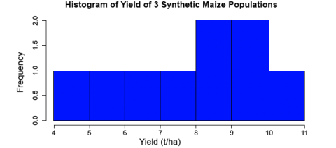
First, let’s look at a histogram of the yield data to see if they follow a normal distribution. We can accomplish this using the hist command.
Enter into the console:
hist(data$Yield, col=”blue”, main=”Histogram of Yield of 3 Synthetic Maize Populations”, xlab=”Yield (t/ha)”, vlab=”Frequency”)
R returns the histogram (Fig. 1) in the Files/Plots/Packages/Help window (bottom-right).
Ex. 1: Create a Boxplot
Let’s go through the command we just entered: data$Yield specifies that we want to plot the values from the column Yield in the data, col=”blue” indicates which color the histogram should be, the entry in quotations after main= indicates the title that you’d like to give the histogram, the entries afterxlab= and ylab= indicate how the x and y axes of the histogram should be labeled. The histogram appears in the bottom-right window in RStudio. The histogram can be saved to your current working directory by clicking ‘export’ on the toolbar at the top of the lower-right window, then clicking “save plot as PNG” or “save plot as a PDF”. You may then select the size dimensions you would like applied to the saved histogram.
Let’s now look at some boxplots of yield by population for this data. First, enter into the Console windowattach(data). The attach command specifies to R which data set we want to work with, and simplifies some of the coding by allowing us just to use the names of columns in the data, i.e. Yield vs.data$Yield. After we enter the attach command, we’ll enter the boxplot command.
attach(data)
boxplot(Yield~Pop, col=”red”, main=”Yield by Population”, xlab=”Synthetic Population”, ylab=”Yield”
R returns the boxplot in the bottom-right window.
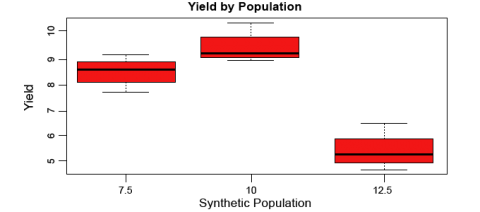
Let’s go through the boxplot command: Yield~Pop indicates that we want boxplots of the yield data for each of the 3 populations in our data, col= indicates the color that we want our boxplots to be, main= indicates the title we want to give the boxplots, and xlab= and ylab= indicate what we want the x and y axes labeled as.
Note: Yield is capitalized in our data file, thus it MUST also be capitalized in the boxplot command.
Ex. 1: Calculate Coefficient of Variance
The coefficient of variance can be calculated for each population in the data set. Looking at the data, we can see that lines 1 to 3 pertain to population 7.5. We know that the coefficient of variation for a sample is the mean of the sample divided by the standard deviation of the sample. By using the command mean(), we can calculate the mean for a sample. Remember that to specify a column from a data frame, we use the $ operator. If we want to calculate the mean of population 7.5 from the data (rows 1 to 3 in the data), we can enter
mean(data$Yield[1:3])
To calculate the standard deviation of the yield for population 7.5, enter
sd(data$Yield[1:3])
The coefficient of variance is therefore calculated by entering
mean(data$Yield[1:3])/sd(data$Yield[1:3])
Ex. 1: Carry Out ANOVA
Now that we’ve gained some intuition about how the data behave, let’s carry out an ANOVA with one factor (Pop) on the data. We first need to specify to R that we want Population to be a factor. Enter into the Console
Pop<-as.factor(Pop)
Let’s go through the command above: as.factor(data$Pop) specifies that we want the Pop column in dataset data to be a factor, which we’ve called Pop.
Now that we have population as a factor, we’re ready to conduct the ANOVA. The model that we are using for this one-factor ANOVA is Yield=Population. In the Console, enter
out <- summary(aov(Yield ~ Pop))
Let’s look at the ANOVA table. Enter out in the Console window.
out
Df Sum Sq Mean Sq F value Pr(>F)
Pop 2 25.537 12.769 19.2 0.00247 **
Residuals 6 3.989 0.665
—
Signif. codes: 0 ‘***’ 0.001 ‘**’ 0.01 ‘*’ 0.05 ‘.’ 0.1 ‘ ‘ 1
Ex. 1: Interpreting the Results
In this ANOVA table, the error row is labeled Residuals. In the second and subsequent columns you see the degrees of freedom for Pop and Residuals (2 and 6), the treatment and error sums of squares (25.537 and 3.989), the treatment mean square of 12.769, the error variance = 0.665, the F ratio and the P value (19.2 and 0.0025). The double asterisks (**) next to the P value indicate that the difference between the yield means of the three populations is significant at 0.1% (i.e., we reject the null hypothesis that the yield means of each population are statistically equivalent). Notice that R does not print the bottom row of the ANOVA table showing the total sum of squares and total degrees of freedom.
R Code Functions
- getwd()
- hist()
- as.factor()
- setwd()
- attach()
- aov()
- read.csv()
- boxplot()
- summary()
- head()
- str()
The Scenario
You are a data analyst for the respected seed company “Vavilov’s Varieties”. In an effort to find a source of genetic resistance to a strain (UG99) of rust that is plaguing the company’s current wheat lines, the company has acquired 300 genetically diverse wheat landraces from central Asia. A test for resistance to the rust strain was done on each of the landraces, and 100 out of the 300 landraces were found to be completely resistant. The company’s plan is to introgress via backcrossing the resistance gene/genes from a single rust-resistant landrace into an elite, high yielding cultivar already being sold by the company. A preliminary yield test with each of the 100 resistant landraces planted in 2 reps at a single location was conducted. Your supervisor wants to know if there is a statistically significant difference among the yield results of the landraces, and if it is therefore possible to minimize yield drag by selecting the highest yielding resistant landrace for use in converting the elite germplasm for resistance to the rust. There are no funds in your budget to acquire commercial statistical software, and in addition your supervisor tells you that he needs to make a decision as soon as possible (precluding you from doing the analysis by hand).
Source Data
You can download the data file here and save it as a .CSV file.
Ex. 2: Enter the Data into R
Do some exploratory analysis on the data (i.e., create a histogram of yield, boxplots for the yield of each landrace, calculate the mean, standard deviation, and coefficient of variation of yield for all of the landraces). Then, carry out an ANOVA with one factor (LR) on the yield data. Finally, explain the results of your analysis in the context of the problem (i.e. does the ANOVA lead you to accept or reject the null hypothesis that the yields of all of the landraces are statistically equivalent). Finally, make a decision as to which landrace should be entered into your company’s wheat breeding program. The R code for this example is almost the same as the Corn Population Example in Activity 8.2. The response variable is still ‘Yield’ and the factor variable is ‘LR’ (landrace).
The following code will assist you in carrying out these analyses.
If you are working in the Script window of R studio, you can enter comments/descriptions on lines of code by first entering the # symbol, then entering your comment after. R will recognize this line as a comment, and not try to execute the line as command when you enter the code from the Script window into the Console using CTRL+ENTER. This can be very useful when working in a team setting where you may have to share code with other team members who might not be familiar with some types of analyses or commands R.
Read the CSV data file into R.
data<-read.csv(“CRD.2.data.csv”, header=T)
Look at the first few lines of the dataset.
head(data)
LR Rep Yield
1 1 1 1.854
2 1 2 1.895
3 2 1 2.157
4 2 2 2.250
5 3 1 1.595
6 3 2 1.777
Create a histogram of the yield data from the dataset.
hist(data$Yield, col=”green”, main=”Histogram of yield of wheat landraces”, xla b=”Yield (t/ha)”,ylab=”Frequency”)
Create a boxplot of the yield for each landrace.
boxplot(data$Yield~data$LR, col=”yellow”, main=”Yield by Population”, xlab=”Landrace”, ylab=”Yield (t/ha)”)
Display the structure of the data frame ‘data’.
str(data)
‘data.frame’: 200 obs. of 3 variables:
$ LR : int 1 1 2 2 3 3 4 4 5 5 …
$ Rep : int 1 2 1 2 1 2 1 2 1 2 …
$ Yield: num 1.85 1.9 2.16 2.25 1.59 …
Make Landrace (LR) a factor by which to separate the yield data
LR <- as.factor(data$LR)
Perform a one-factor ANOVA
out <- summary(aov(Yield ~ LR))
out
Df Sum Sq Mean Sq F value Pr(>F)
LR 99 9.721 0.09819 2.997 4.71e-08 ***
Residuals 100 3.276 0.03276
—
Signif. codes: 0 ‘***’ 0.001 ‘**’ 0.01 ‘*’ 0.05 ‘.’ 0.1 ‘ ‘ 1
Ex. 2: Interpret the ANOVA
Now, let’s interpret the results of the ANOVA.
The P value is given in the ANOVA table as 4.65e-08, or 0.0000000465. Looking at the significance codes at the bottom of the ANOVA table output in R, we can see that this p-value is significant at even the most stringent of significance level (0.001). This leads us to reject the null hypothesis that the yields of the different landraces are statistically the same. What does this mean for us as plant breeders? If the yields of the different landraces are not all statistically equivalent, then there must be some landraces that have higher mean yields than others. We can therefore select the top performing landrace for yield to minimize the effect of yield drag when introgressing the gene/s that confer resistance to rust strain UG99 into an elite background.
The Linear Additive Model
A way to conceptualize how treatments, such as plant density or fertilizer, affect crop yields is to write the yield (Y) as composed of an overall mean, a treatment effect, and error. The common way to express this is in the form of a linear model equation.
Later we will use this linear model equation method for understanding more complex situations and experiments. It is important to realize that every designed experiment can be described by a linear additive model and that this model determines the manner in which we apply the ANOVA to the experiment. The linear additive model lists all the sources of variation that are accounted for in the experiment relative to the overall mean. For the one-way analysis of variance, the ANOVA table contains two sources: treatments and error. In experiments containing additional treatments as factors, there will be more sources in the model and these will correspond to additional rows in the ANOVA table.
The Linear Model Equation
As discussed in the previous sections, the ANOVA decomposes the variability for each part of the experiment. Each effect can be considered as a part of the variability seen in each experimental unit. Since these effects are additive, we can view the result from each unit as a combination of each effect. Symbolically, the linear additive model for ANOVA is:
[latex]Y_{ij} = \mu + T_{i} + \epsilon_{({i})j}[/latex]
[latex]\text{Equation 5 Linear model for ANOVA}[/latex].
where:
Yij = response observed for the ijth experimental unit
 = overall population mean
Ti = effect of the ith treatment
 = effect associated with the ijth experimental unit, commonly referred to as error or residual
About these subscripts: “i” refers to the treatment, and “j” refers to the replication of that treatment. So an experiment will have “i*j” experimental units; each unit will be identified by a unique “ij” combination. For example, the response of experimental unit with the 4th replication of the 3rd treatment will be notated as Y34.
This is the same as the linear model for the t-test, expanded to more than just two treatments or populations.
Application
For the corn population experiment we can rewrite the model to indicate the true sources of variation as:
[latex]Yield_{ij} = \mu + POP_{i} + PLOT_{({i})j}[/latex]
[latex]\text{Equation 6 Linear model for ANOVA with true sources of variation}[/latex].
where:
Yieldij = corn yield for the ijth plot
= average corn yield for the experiment
POPi = effect of the ith planting population
PLOT(i)j = effect associated with the ijth plot (residual)
You can think of a linear model as a ledger. The dependent variable (Yij) is analogous to the current balance and the mean can be thought of as the initial balance. Each of the other terms (independent variables) are either a credit or a debit. So, in the model above, corn yield in a given plot is simply the value that remains after the average yield has been adjusted for the effects of population and error.
Summary
ANOVA
- Tests hypothesis that treatment means are same.
- Compares variance from treatment mean differences with that from error.
- Separates the variances in a table, with sources being Treatment, Error, and Total.
- Has degrees of freedom (df) for each source of variation.
- Has sum of squares (SS) for each source.
- Computes variance estimates as mean squares, ms = ss/df.
F-test
- The null hypothesis (no difference in treatment means) is tested with the F-ratio,F = Treatment MS/Error MS.
- For each alpha level, the table F – value depends on numerator and denominator df.
Linear Additive Model
- Expresses the partition of Y into overall mean, treatment, and error.
- These components are added to get Y.
- Provides basis for more complex linear models in later units.
How to cite this chapter: Moore, K., R. Mowers, M.L. Harbur, L. Merrick, A. A. Mahama, & W. Suza. 2023. The Analysis of Variance (ANOVA). In W. P. Suza, & K. R. Lamkey (Eds.), Quantitative Methods. Iowa State University Digital Press.
definition
Often abbreviated to ANOVA, a general term for a set of statistical procedures to differentiate treatment effects by separating combined variability in an experiment
A procedure or manipulation for which you wish to measure a response. Some good agronomic examples are the application of specific fertilizer rates and the planting of specific crop varieties for the purposes of comparison.
That variability in an experiment that is random or cannot be explained.
