
Chapter 13: Multiple Regression
Ron Mowers; Dennis Todey; Ken Moore; Laura Merrick; Anthony Assibi Mahama; and Walter Suza
Observing Variables
In Chapter 7 on Linear Correlation, Regression, and Prediction, we discussed determining the correlation and possible regression relationships between an independent variable X and a dependent variable Y. Specifically, in regression, the discussion was based on how the change in one variable (X) produced an effect on another (Y). This is the essence of regression. But from experience, we know that often multiple causes interact to produce a certain result. For example, yield from a crop is based on the amount of water a plant has to use, the soil fertility of the field, the potential of the seed to produce a plant, pest and pathogen pressures, and numerous other factors. In this lesson, we’ll explore how we can determine linear relationships between multiple independent variables and a single dependent variable.
Exploring Multiple Variables
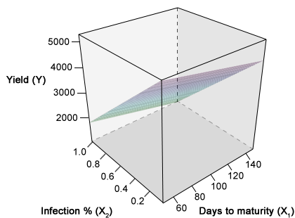
Multiple regression functionally relates several continuous independent variables to one dependent variable. In the above example, barley yield per plot (Y) is shown as a function of the percentage of plants in the plot affected by rust (X1) and the days to maturity required by the cultivar grown in a particular plot (X2). Yield is modeled as a linear combination of these two X variables in the response surface on the previous slide. Before we can relate the dependent variable Y to the independent X variables, we need to know the interrelationships between all of the variables. Multiple correlation and partial correlation provide measures of the linear relationship among the variables.
Separating the individual factor’s effect on the whole result, such as the effect of rust infection or the number of days a particular cultivar requires to reach maturity, can be difficult and, at times, confounding. The objective of this chapter is to explain and illustrate the principles discussed in Chapter 7 on Linear Correlation, Regression and Prediction or correlating two variables or enumerating the effect of one variable on another, but now expanded to multiple variables.
- To define correlation relationships among several variables
- To separate the individual relationships of multiple independent variables with a dependent variable
- To test the significance of multiple independent variables and to determine their usefulness in regression analysis
- To recognize some of the potential problems resulting from improper regression analysis
Multiple Correlation and Regression
The correlation of multiple variables is similar to the correlation between two variables. The same assumptions apply; the sampled Y’s should be independent and of equal variance. Error (variance) is associated with the Y’s while X’s have no error, or the error is small. But now, since there are multiple factors involved, the correlations are somewhat more complex, and interactions between the Xi variables are expected. A note on notation: We now include a subscript with the “X” to indicate which independent variable to which we are referring. Three levels of correlation are used in determining the multi-faceted relationships; simple correlation, partial correlation, and total correlation.
Simple Correlation
The simple correlation between one of the Xi‘s and Y is computed for a simple correlation of X and Y. This calculation assumes a direct relationship between the particular Xi and Y. It is also useful in stating the simple relationship between two Xi‘s in the multiple correlation. When determining the significance of regression coefficients, the variable with the largest simple correlation with Y is usually the starting point. Some interaction among numerous X and Y variables is likely to occur. Because two Xi‘s have large simple correlations with a resulting Y does not necessarily indicate that their relationships to Y are independent of each other. They may be measuring the same effect on Y. The number of hours of sunlight (cloud-free skies) and GDDs both have a good (simple) correlation to the rate of crop development. But their effects would not be additive. There would be a significant interaction between these two variables in describing crop development. The two variables measure two different factors, light and temperature. However, the amount of sunlight and temperature are generally highly correlated during the summer. So there would be a significant relationship between the two variables. These individual effects can be separated using partial correlation.
Partial Correlation
Quantifying which continuous X variables are best correlated with the continuous Y-variable requires an understanding of the interactions between the Xi‘s. To break down the interaction requires partial correlation coefficients. These use the simple correlation coefficients to explain the correlation of two variables with all other variables held constant. One such example is, “How much yield will result from nitrogen applications assuming the seasonal amount of rainfall will be average?” Here, rainfall is held constant, and the effect of nitrogen on yield would be used for a partial correlation. This relationship is given for the partial coefficient of determination between Y and X1 where two X’s are involved, as shown in Equation 1.
[latex]r_{YX_{1}X_{2}} =\frac{r_{YX_1}-r_{YX_2}r_{X_1X_2}}{\sqrt{1-r^2_{YX_2}}\sqrt{1-r^2_{YX_1}}}[/latex].
[latex]\textrm{Equation 1}[/latex] Formula for calculating partial coefficient of determination between Y and X.
where:
[latex]\small X_1, X_2[/latex] = continuous variables X,
[latex]\small Y[/latex] = continuous variable Y,
[latex]r[/latex] = correlation coefficient.
To calculate the partial coefficient of determination between Y and X2, just reverse the equation, i.e. use rYX1 and vice versa. Don’t panic! You will not be asked to hand-calculate this on the homework or exam. That is why we use R!
Correlation Matrix
The value rYX1 is the simple correlation between Y and X1. The whole equation describes the correlation between Y and X1 with X2 held constant. The relationship between the X1 and Y is displayed within the effect of the interaction. Partial correlations can be calculated for all variables involved. They can also be calculated for more than three variables, but the equation becomes more complex. Often, the total and partial correlations are calculated and displayed in a table with the individual Xis and Y listed across the top and down the left side. The correlations for each variable pair are displayed at the intersection of the variables.
| n/a | X1 | X2 | Y |
|---|---|---|---|
| X1 | 1 | 0.462 | 0.693 |
| X2 | 0.462 | 1 | 0.354 |
| Y | 0.693 | 0.354 | 1 |
Total Correlation
The combination of these partial effects leads to a multiple correlation coefficient, R, which states how related the Y is to the combined effects of the Xi‘s. For X1, X2, and Y, the total correlation is determined once again using the simple correlations (Equation 2):
[latex]R^{2}_{Y\cdot X_{1}X_{2}} =\frac{r^{2}_{YX_1}+r^{2}_{YX_2}-2r_{YX_1}r_{YX_2}r_{Y_1X_2}}{1-r^{2}_{X_1X_2}}[/latex].
[latex]\textrm{Equation 2}[/latex] Formula for calculating multiple correlation coefficient, R.
In this equation,[latex]r^2_{YX_1}[/latex] and [latex]r^2_{YX_2}[/latex] are just the squares of partial correlation coefficients.
The calculations for 2 Xi‘s are relatively straightforward, but for three or more variables, the calculations involve a large number of terms with different correlations among individual variables. Consequently, total correlation is calculated with computer programs, such as R.
Similar to the linear correlation coefficient, the total correlation coefficient, when squared, produces the multiple coefficient of determination, R2. This value explains the proportion of the Y variation, which can be accounted for by a multiple regression relationship. The partial correlation coefficients squared produce the partial coefficients of determination, r2, or that proportion of variance which can be described by one variable, while the partial coefficients will be used in testing individual regression coefficients for significance.
Calculating the Correlation
Graphing data to visualize the correlation relationships in multiple dimensions is difficult. The graphing of data involving 2 Xi‘s with Y is possible in 3-dimensional space. Using the variables mentioned, the regression equation would be a plane in the X1, X2, Y space (Fig. 1). The partial regression coefficients for X1 with Y and X2 with Y in this space could be used to produce lines where the plane intersected a certain X value. For example, the following equation would produce a plane on a graph.
[latex]\small \textrm{Y}=2.4X_1+3.9X_2-7.1[/latex].
Setting X1 equal to 0 would reduce the above equation of a plane to a linear equation:
[latex]\small \textrm{Y}=3.9X_2-7.1[/latex].
Either X1 or X2 could be set to any value producing any number of different linear relationships in the plane. With more than two X values, graphing the relationship in 3 dimensions is not easily done. Instead of graphing, interpreting the data numerically and conceptually is the preferred method.
Ex. 1, Step 1
R CODE FUNCTIONS
- cor
- cor.test
- install.packages
- library
- pcor
Multiple regression functionally relates several continuous independent variables (X), to one dependent variable, Y. For example, we could carry out multiple regression with yield as the dependent response variable (Y), X1 as an independent variable indicating the amount of fertilizer applied and X2 as an independent variable indicating the amount of water each plot received. In this example, we model yield as a linear combination of the amount of water and fertilizer applied to each plot in multiple regression. However, before we can relate Y to the other variables, we need to know the interrelationships of all the variables. Multiple correlation provide measures of the linear relationship among variables.
head(data)
cor(data$perc.inf, data$Yield)
cor(data$perc.inf, data$Yield)
R returns the simple correlation matrix.
dtm perc.inf yield
dtm 1.00000000 0.00352555 -0.2268896
perc.inf 0.00352555 1.00000000 -0.9475068
yield -0.22688955 -0.94750681 1.0000000
Great! Now we have the simple correlation matrix showing the correlations between RIL (Line), days to maturity (dtm), infection rate (perc.inf), and yield. The correlation matrix returned by R is constructed with the variables listed as both row and column headings. The top number at the intersection of a row and column is the correlation coefficient for those two variables. For example, the simple correlation between yield and perc.inf is -0.94750681.
Ex. 1, Step 2
First, calculate the p-value for the simple correlation of perc.inf and yield.
data<-read.csv(“barley.csv”, header = T)
R returns
Pearson’s product-moment correlation
data: data$perc.inf and data$yield
t = -29.3362, df = 98, p-value < 2.2e-16
alternative hypothesis: true correlation is not equal to 0
95 percent confidence interval:
-0.9644361 -0.9228353
sample estimates:
cor
-0.9475068
The p-value for the correlation between perc.inf and Yield is 2.2*10-16, which is extremely low. This low p-value tells us that the correlation between the two variables (yield and perc.inf) is highly significant.
Ex. 1, Step 3
Now, let’s calculate the p-value for the correlation of dtm and yield.
cor.test(data$dtm, data$yield)
R returns
Pearson’s product-moment correlation
data: data$dtm and data$yield
t = -2.3062, df = 98, p-value = 0.0232
alternative hypothesis: true correlation is not equal to 0
95 percent confidence interval:
-0.40524772 -0.03189274
sample estimates:
cor
-0.2268896
The p-value, though not as low as that which was calculated for the correlation between perc.inf and Yield, is still significant at =0.05. Thus, the correlation between dtm and yield is also significant. Now let’s see if there is a significant p-value for the correlation of perc.inf and DTM (the two X variables).
Ex. 1, Step 4
Calculate the p-value for the correlation between DTM and perc.inf.
cor.test(data$dtm, data$perc.inf)
R returns
Pearson’s product-moment correlation
data: data$dtm and data$perc.inf
t = 0.0349, df = 98, p-value = 0.9722
alternative hypothesis: true correlation is not equal to 0
95 percent confidence interval:
-0.41930262 -0.1998053
sample estimates:
cor
0.00352555
Based on the extremely high p-value, the correlation between perc.inf and DTM is not significant.
Ex. 1, Step 5
Interpret the results:
Which of the variables are the most correlated? Which will contribute the most to the final regression of yield on dtm and infection rate perc.inf? The first question can be answered by looking at the simple correlation matrix that we created in step 5. perc.inf and yield have a simple correlation of -0.94750681, and dtm and yield have a simple correlation of -0.22688955. The correlation of dtm and yield has a smaller absolute magnitude. Thus, infection rate (perc.inf) will contribute the most to the regression equation when we calculate it.
Before we construct a regression model for yield, we need to analyze how days to maturity (dtm) interact with infection rate (perc.inf) in the multiple regression. Despite the simple correlation between dtm and perc.inf being not statistically significant, calculating the partial correlation between these two variables may help explain a possible relationship between them. Simple correlations are the basis for calculating the additional correlation relationships.
Ex. 1, Step 6
Now, let’s calculate the partial correlation matrix for the 3 variables. To do this, we’ll first need to get the package ‘ppcor’.
Install.packages(‘ppcor’)
library (ppcor)
ppcor(data)
R returns
$estimate
dtm perc.inf yield
dtm 1.0000000 -0.6790490 -0.6991729
perc.inf -0.6790490 1.0000000 -0.9720637
yield -0.6991729 -0.9720637 1.0000000
$p.value
dtm perc.inf yield
dtm 0.000000e+00 8.210329e-20 5.887334e-22
perc.inf 8.210329e-20 0.000000e+00 0.000000e+00
yield 5.887334e-22 0.000000e+00 0.000000e+00
$statistic
dtm perc.inf yield
dtm 0.000000 -9.110368 -9.631483
perc.inf -9.110368 0.000000 -40.788323
yield -9.631483 -40.788323 0.000000
Note: Using the pcorr function, we obtain test statistics (t) and p-values without having to use any other function, such as cor.test. The R output $estimate gives the partial correlations, where one of the 3 variables is held constant as a partial variable. For example, the partial correlation of yield and perc.inf is -0.9720637; dtm is held constant as a partial variable for this correlation. The p-value for this correlation, or the probability of the correlation equal to zero, is so small that R returns a p-value of 0. From this incredibly small p-value, we would conclude there is a significant correlation between yield and organic perc.inf. The partial correlation coefficient between yield and dtm is -0.6991729, and the probability of this correlation being equal to zero is only 5.887334e-22. Thus, we would conclude that dtm is very much correlated with the yield, at least under these disease conditions.
Did the partial correlation follow the simple correlation in magnitude? The partial correlation of dtm with yield (with perc.inf held constant) was -0.6991729, while that of perc.inf with yield (dtm held constant) is -0.9720637. The squared values of the partial coefficients of determination are used in calculating the contribution of each variable to the regression analysis. These values are calculated as in equation 2 from above for the simplest case of multiple regression, where there are two X’s and one Y. More complex equations result from equations with more than two X variables.
- Set your working directory to the folder containing the data file barley.csv
- Read the file into the R data frame, calling it data.
data<-read.csv(“barley.csv”, header=T)
- Check the head of the data to make sure it was read in correctly.
- Calculate the correlation between the fusarium infection rate (perc.inf) and barley yield.
- Calculate the correlation between DTM and yield.
- Install the package ‘ppcor’.
- Load the package.
- Calculate the partial correlation between yield, dtm, and perc.inf.
Multiple Regression
Relationships Among Multiple Variables
Multiple regression determines the nature of relationships among multiple variables. The resulting Y is based on the effect of several X’s (Equation 3). How much of an effect each has must be quantified to determine the equation (below). The degree of effect each X has on the Y is related through partial regression coefficients. The b-value estimate of each regression coefficient can be determined by solving simultaneous equations. Usually, computer programs determine these coefficients from the data supplied.
[latex]\normalsize \textrm{Y}=a + b_1x_1 + b_2x_2 + ... + b_ix_i + \epsilon[/latex].
[latex]\textrm{Equation 3}[/latex] Formula for calculating multiple regression for the relationship among multiple variables.
where:
[latex]a[/latex] = the [latex]\small Y[/latex] intercept,
[latex]b[/latex] = estimates of the true partial regression coefficients, β.
The [latex]a[/latex] is the Y-intercept, or Y estimate, when all of the X’s are 0. The [latex]b's[/latex] are estimates of the true partial regression coefficients β, the weighting of each variable’s effect on the resulting Y. The b’s are interpreted as the effect of a change in that X variable on Y, assuming the other X’s are held constant. These can be tested for significance. The weighting of effects now will be based on regression techniques.
The simplest example of multiple linear regression is where two X’s are used in the regression. The technique of estimating b1 and b2 minimizes the error sums of squares of the actual from estimated Y’s. The variability of the data (Y’s) can be partitioned into that caused by different X variables or into error.
Example of Multiple Correlation and Regression
The simplest example of multiple correlation involves two X’s. Calculations with more variables follow a similar method but become more complex. Computer programs have eased the computational problems. Proper analysis of the data and interpretation of analyses are still necessary and follow similar procedures.
The following two-variable research data were gathered relating the yield of inbred maize to the amount of nitrogen applied and the seasonal rainfall data (Table 2).
| Yield of Maize
bu/Ac |
Fertilizer
lb N/Ac |
Rainfall
in. |
|---|---|---|
| 50 | 5 | 5 |
| 57 | 10 | 10 |
| 60 | 12 | 15 |
| 62 | 18 | 20 |
| 63 | 25 | 25 |
| 65 | 30 | 25 |
| 68 | 36 | 30 |
| 70 | 40 | 30 |
| 69 | 45 | 25 |
| 66 | 48 | 30 |
Review the Data
The first issue is to review how highly correlated the data are. Since visualization of multiple data is more difficult, numerical relationships must be emphasized. The first step is to examine the correlations among the variables. The simple correlations (calculated as in Chapter 7 on Linear Correlation, Regression and Prediction) may be computed for the three variables (see below).
Simple Correlations
[latex]\small r_{YX_1} = 0.895 \\ \small r_{YX_2} = 0.944 \\ \small r_{X_1X_2} = 0.905[/latex]
Partial Coefficients of Determination
All are highly correlated. But these simple correlations include the interactions among variables. To determine individual relationships, calculations of partial coefficients of determination are helpful (Equation 4).
[latex]r^2_{YX_1 \dot{}X_2} = \frac{(r_{YX_1} - r_{YX_2}r_{X_1X_2})}{(1 - r^2_{X_1X_2})(1-r^2_{X_1X_2})} = \small 0.081[/latex]
[latex]r^2_{YX_2 \dot{} X_1} = \small 0.499[/latex]
[latex]r^2_{YX_2 \dot{} X} = \small 0.170[/latex]
[latex]\textrm{Equation 4}[/latex] Example calculation of partial coefficient of determination.
These values are the additional variability that can be explained by a variable, such as that by X1, after the variability of X2 alone has been accounted for. These values are used in computing the ANOVA for multiple regression. The partial correlations may be found by taking the square root of these partial coefficients of determination.
Total Coefficients of Determination
The R2-value is the total coefficient of determination, which combines the X’s to describe how well their combined effects are associated with the Y’s. This is determined as shown below (Equation 5).
[latex]R^2_{Y \dot{}X_1X_2} = \frac{0.801+0.891-2(0.895)(0.944)(0.905)}{1-0.819} = \small 0.900[/latex]
[latex]\textrm{Equation 5}[/latex] Example calculation of total coefficient of determination.
The R2 value is the proportion of variance in Y that is explained by the regression equation. This can be used to partition the variability in the ANOVA. The square root of this value gives the correlation of the X’s with Y. It is obvious that the correlations are not additive. The simple correlations are all greater than 0.8, and the correlation between X1 and X2 is 0.905. This is where partial correlation comes into play.
Partial Regression Coefficients
Before we can create an ANOVA and test the regression, we need a regression equation as determined by R. The estimate of the regression relationship is found to be in the below equation.
[latex]\small \textrm{Y}= 49.53 + 0.089x_1 + 0.515x_2[/latex].
The partial regression coefficients indicate that for the data gathered here, each additional pound of nitrogen applied per acre would produce an additional 0.089 bushels of maize per acre, and for each additional inch of rainfall, an additional 0.516 bushels per acre. An estimate of the yield is determined by entering the amount of nitrogen applied to the field and the amount of rainfall into the equation. The number produced is the regression equation estimate of the yield based on the data gathered.
The next issue is deciding if this equation is useful and explains the relationship in the gathered data. The sums of squares are partitioned in an ANOVA table, and the significance of the regression equation as a whole and the individual regression coefficient estimates are tested for significance in the next section.
Ex. 2: Multiple Regression and Anova Using R (1)
This exercise contains 26 steps (including this statement).
Ex. 2: Multiple Regression and Anova Using R (2)
R CODE FUNCTIONS
- anova
- summary
- lm
- pf
- ppcor
Multiple regression is used to determine the nature of relationships among multiple variables. The response variable (Y) is defined as the product of the effects of several explanatory variables (X’s). The level of effect each X has on the Y variable must be quantified before a regression equation can be constructed (i.e. equation 3). The degree of effect each X has on the Y is related through partial regression coefficients. The coefficient estimate of each explanatory variable can be determined by solving simultaneous equations. Usually, computer programs such as R determine these coefficients from the data supplied, [latex]\small \textrm{Y}=a + b_1X_1 + b_2X_2 + ... + b_iX_i + \epsilon[/latex].
In equation 3 above, the a term is the Y-intercept, or the estimate of Y when all of the X’s are 0. The b with each X is an estimate of the true partial regression coefficient ß for that X variable, the weighting of each variable’s effect on the resulting Y. The b’s are interpreted as the effect of a change in that X variable on Y, assuming the other X’s are held constant. These coefficients can also be tested for significance. The weighting of effects will now be based on regression techniques.
The simplest example of multiple linear regression is where two X variables are used in the regression. The technique of estimating b1 and b2 via multiple regression minimizes the error sums of squares of the actual data from the estimated Y’s. The variability in the data can be partitioned into that which is caused by different X variables or that which is caused by error.
In the file QM-Mod13-ex2.csv, we have yield data from one inbred maize line under all factorial combinations of 9 different levels of nitrogen treatment and 9 different levels of drought treatment. We’ll use these data to investigate correlations between the variables, to do a multiple regression analysis, and to carry out an analysis of variance (ANOVA).
Ex. 2: Multiple Regression and Anova Using R (3)
Read the dataset into R, and have a look at the structure of the data.
data<-read.csv(“ex2_data.csv”, header=T)
head(data)
R returns
drought N yield
1 -4 0 1886.792
2 -4 28.025 2590.756
3 -4 56.05 3743.000
4 -4 84.075 4910.937
5 -4 112.1 5656.499
6 -4 140.125 5689.165
The data contain entries for yield (kg/ha), level of nitrogen applied (kg/ha), and a “drought” score to indicate the level of drought stress applied (i.e. a level of -4 is the maximum drought stress applied, and a value of 4 is the minimum level of drought stress).
Note: Even though we have fixed treatments assigned to each test plot, we will run the analyses in this ALM as if they were random treatments (i.e. keeping the values for drought and N as numeric). This will allow us to investigate simple and partial correlations.
Ex. 2: Multiple Regression and Anova (4)
Simple Correlation
The correlation between X and Y, ([latex]\small P_{XY}[/latex]), is calculated as the covariance of X and Y divided by the product of the standard deviations of X and Y, i.e., [latex]\small P_{XY}=\frac{cov(X,Y)}{\sigma_{X}\sigma_{Y}}[/latex]
The first step is to review how highly correlated the data are. Since visualization of multiple data is more difficult, numerical relationships must be emphasized. Let’s examine the correlations among the variables. Calculate the simple correlations between the 3 variables by entering into the console window.
cor(data)
R returns the simple correlations matrix
drought N yield
drought 1.0000000 0.0000000 0.7364989
N 0.0000000 1.0000000 0.2147159
yield 0.7364989 0.2147159 1.0000000
Ex. 2: Multiple Regression and Anova Using R (5)
Partial Correlation
Taking X1 to be nitrogen, X2 to be drought, and Y to be yield, we can list the simple correlation variables.
Simple Correlations
[latex]\small r_{YX_{1}}=0.2147159 \\ \small r_{YX_{1}}=0.7364989 \\ \small r_{Y_1X_{2}}=0[/latex]
Both nitrogen and irrigation are correlated with yield, but these simple correlations include interactions among the variables. To determine individual relationships, calculations of partial correlation coefficients are helpful. Partial correlation coefficient values are the additional variability in the response variable that can be explained by an independent variable, such as that by X1, after the variability of another independent variable, such as X2, alone has been accounted for. These values are also used in computing the ANOVA for multiple regression.
We will now do a quick investigation of the partial correlations between the variables in the dataset. If you haven’t already, load the ‘ppcor’ package. Then, use the pcor command to obtain the matrix of partial correlations between all variables in the data set.
library(ppcor)
pcor(data)
Ex. 2: Multiple Regression and Anova Using R (6)
R returns 3 matrices: a matrix with the partial correlation coefficient estimates ($estimate), a matrix with the test statistic for the estimate ($statistic), and a matrix for the p-value of the test statistic ($p.value).
$estimate
drought N yield
dtm 1.0000000 -0.239363 0.7540868
N -0.2393630 1.000000 0.3174210
yield 0.7540868 0.317421 1.0000000
$p.value
drought N yield
drought 0.000000e+00 0.029458897 3.658519e-24
N 2.945890e-02 0.000000000 3.113831e-03
yield 3.658519e-22 0.003113831 0.000000e+00
$statistic
drought N yield
dtm 0.000000 -2.177291 10.140333
perc.inf -2.177291 0.000000 2.956271
yield 10.140333 2.9562
Ex. 2: Multiple Regression and Anova Using R (7)
Let us calculate the partial correlation coefficient for nitrogen on yield by hand, using Equation 1, to check the calculation returned by R in the estimate matrix.
[latex]r_{YX_{1}X_{2}} =\frac{r_{YX_1}-r_{YX_2}r_{X_1X_2}}{\sqrt{1-r^2_{YX_2}}\sqrt{1-r^2_{YX_1}}}[/latex]
[latex]r_{YX_{1}X_{2}} =\frac{(0.2147159-0.7364989*0)}{\sqrt{(1-0.7364989^2)(1-0)}}=\frac{0.2147159}{0.6764387}=\small 0.317421[/latex].
You can see that the value in the estimate matrix for the partial correlation coefficient between nitrogen and yield is identical to the value obtained by our hand calculation. Also, based on the p-value matrix, all of the partial-correlation estimates are statistically significant.
The test-statistic matrix contains values calculated from the standard normal distribution (with a mean of 0 and standard deviation of 1). The test statistic for the partial correlation of nitrogen on yield is 12.12521. We can check that this value is correct by calculating the p-value for this value from the standard normal distribution by entering
(1-pnorm(2.95621, mean=0, sd=1))*2
Ex. 2: Multiple Regression and Anova Using R (8)
R returns
[1]0.00311834
The p-value for the partial correlation coefficient given in the R output from calculating the partial correlation coefficients is identical to that given in the R output using the pcor function.
The R2 value is the total coefficient of determination, which combines the explanatory variables (X’s) to describe how well their combined effects are associated with the response variable (Y). This is determined by the following equation:
[latex]R^2_{Y \dot{}X_1X_2} = \frac{r^2_{YX_1} + r^2_{YX_2} - 2r_{YX_1}r_{YX_2}r_{X_1X_2}}{1-r^2_{X_1X_2}}[/latex]
The R2 is very useful for interpreting how well a regression model fits. Its value is the proportion of variance in Y that is explained by the regression equation. The closer to 1.0, the better the fit; a value of 1 would mean all of the data points fall on the regression line. The square root of this value gives the correlation of the X’s with Y. It is obvious that the correlations are not additive. This is where partial correlation comes into play.
Ex. 2: Multiple Regression and Anova Using R (9)
The drawback of relying on the R2 value as a measure of fit for a model is that the value of R2 increases with each additional term added to the regression model, regardless of how important the term is in predicting the value of the dependent variable. The Adjusted R2 value (or R2Adj) is a way to correct for this modeling issue. The formula for Adjusted R2 is:
[latex]R^2_{Adj}=1-\frac{(1-R^2)-(N-1)}{n-K-1}[/latex].
where R2 is the regression coefficient, n is the sample size, and k is the number of terms in the regression model. The R-squared value increases with each additional term added to the regression model, so taken by itself, can be misleading. The R2Adj takes this into account and is used to balance the cost of adding more terms; i.e. it penalizes the R2 for each additional term (k) in the model. The R2Adj value is most important for comparing and selecting from a set of models with different numbers of regression terms. It is not of great concern until you are faced with choosing one model to describe a relationship over another. We’ll carry out hand calculations for both R2 and R2Adj after we run the regression in R.
Ex. 2: Multiple Regression and Anova Using R (10)
Regression Model Significance
The initial test is to determine if the total regression equation is significant. As in linear regression, “does the regression relationship explain enough of the variability in the response variable to be significant?”
The testing of the regression equation partitions the total sum of squares using the total coefficient of determination, R2. Note that this is not the same as the square of total correlation.
[latex]\small R^2_{Adj}={\dfrac{\text{(Regression SS)}}{\text{ Total SS}}}[/latex].
Initially, the null hypothesis being tested is that the whole regression relationship is not significantly different from 0.
[latex]\small H_{0}:\beta _{1}=\beta _{2}=0 \\ \small H_{a}:\beta _{1} = \beta _{2}\neq 0[/latex]
Ex. 2: Multiple Regression and Anova Using R (11)
The F-test for multiple linear regression uses the regression mean square to determine the amount of variability explained by the whole regression equation. If the regression mean square is significant at your specified level, the null hypothesis that all of the regression coefficients are equal to 0 is rejected. This F-test does not differentiate between coefficients; all are significant, or none are according to the test.
Individual regression coefficients (b1, b2, etc.) may be tested for significance. The simple coefficient of determination between each X and Y explains the sum of squares associated with each regression coefficient, including interactions with other X’s. The partial coefficient of determination between each X and Y explains the additional variability without interaction. These can be tested with the residual error not explained by the regression model to test the significance of each X.
Each coefficient may also be tested with a t-test; R does this automatically when you run a multiple regression model using the lm function.
Ex. 2: Multiple Regression and Anova Using R (12)
MULTI-LINEAR REGRESSION
Let’s run a multiple regression analysis where yield is the response variable and drought and nitrogen are the explanatory variables. We will keep nitrogen and drought as numeric variables for this analysis but later will run the same analysis with these variables as factors.
In the console window, enter
summary(1m(data=data,yield~drought+N))
Let’s go through this command from the inside out.
- data = data indicates that we want to run the linear model with dataset ‘data’
- yield~ drought + N specifies that the regression equation we are analyzing is yield = ‘the amount of nitrogen applied’ + ‘the amount of drought applied’
- lm indicates to R that we want to run a linear regression model
- Summary indicates that we want R to return all of the useful information from the regression analysis back to us.
Ex. 2: Multiple Regression and Anova Using R (13)
R returns
Call:
lm(formula = yield ~ drought + N, data = data)
Residuals:
Min IQ Median 3Q Max
-4204.2 -1118.0 1.8 1251.6 3148.9
Coefficients:
Estimate Std. Error t value Pr(>|t|)
(Intercept) 7829.436 363.787 21.522 <2e-16 ***
drought 774.828 76.410 10.140 6.78e-16 ***
N 8.060 2.727 2.956 0.00412 ***
—
Signif. codes:
0 ‘***’ 0.001 ‘**’ 001 ‘*’ 0.05 ‘.’ 0.1 ‘ ‘ 1
Residual standard error: 1776 on 78 degrees of freedom
Multiple R-squared: 0.5885,
Adjusted R-squared: 0.578
F-statistic: 55.78 on 2 and 78 DF, p-value: 9.1e-16
Ex. 2: Multiple Regression and Anova Using R (14)
The R2 value is given at the bottom of the R output as 0.5885. This means that the model explains 58.85% of the variation in yield. Let’s calculate the R2 value by hand using the simple correlation coefficient matrix from above (Equation 2).
[latex]R^2_{Y \cdot{} X_1 X_2} = \frac{r^2_{YX_1}+r^2_{YX_2}-2r_{YX_1}r_{YX_2}r_{X_1X_2}}{1-r^2_{X_1X_2}}[/latex]
[latex]{R^2_{Y \cdot{}X_1X_2}}=\frac{0.2147159^2+0.7364989^2-2(0.2147159)(0.7364989)(0)}{1-0} = \small 0.5885[/latex]
The value obtained for R2 obtained by our hand calculation is identical to the value returned by R.
Now, let’s calculate the [latex]R^2_{Adj}[/latex]for the model by hand. Use the value of R2 from the R output (0.5885).
[latex]R^2_{Adj}=1-\frac{(1-R^2)-(N-1)}{n-K-1}[/latex] = [latex]1-\frac{(1-0.5885)-(80-1)}{(80-2-1)}=\small 0.5778117\sim 0.578[/latex].
This is the same value for [latex]R^2_{Adj}[/latex] as given in the R output (under “Adjusted R-squared”).
Ex. 2: Multiple Regression and Anova Using R (15)
VARIABLE INTERACTION
Should we include a term in the linear model indicating the interaction between nitrogen and drought? Let’s run the regression again, this time adding a variable accounting for the interaction between the two independent variables into the model. (i.e. the amounts of drought and nitrogen applied). The interaction variable is specified using a multiplication sign (*) with the explanatory variables that you are analyzing for interaction.
summary(1m(data=data,yield~N+drought+N*drought))
Ex. 2: Multiple Regression and Anova Using R (16)
R returns
Call:
lm(formula = yield ~ N + drought + N * drought, data = data)
Residuals:
Min IQ Median 3Q Max
-3857.9 -1076.4 22.8 1244.8 3148.9
Coefficients:
Estimate Std. Error t value Pr(<|t|)
(Intercept) 7829.436 364.898 21.457 < 2e-16 ***
N 8.060 2.735 2.947 0.00424 **
drought 688.736 141.324 4.873 5.75e-06 ***
N:drought 0.768 1.059 0.725 0.47061
—
signif. codes:
0 ‘***’ 0.001 ‘**’ 0.01 ‘*’ 0.05 ‘.’ 0.1 ‘ ‘ 1
Residual standard error: 1781 on 77 degrees of freedom
Multiple R-squared: 0.5913
Adjusted R-squared: 0.5754
F-statistic: 37.14 on 3 and 77 DF, p-value: 5.986e-15
Ex. 2: Multiple Regression and Anova Using R (17)
Compare the R2Adj value and the F-statistic of the model, including the interaction, to the model not including the interaction. Which model fits the data better?
With interaction: R2Adj = 0.5754, F = 37.14
Without interaction: R2Adj = 0.578, F = 55.78
The model without the interaction between Nitrogen and Irrigation has a slightly better fit for these data than the model including the interaction. Also, the regression coefficient on the interaction term has a very high p-value, indicating that is not statistically significant. Save the model without the interaction as ‘m1’.
m1<-1m(data=data,yield~N+drought)
Ex. 2: Multiple Regression and Anova Using R (18)
Calculate the ANOVA table for the multiple regression models with and without the interaction between N and drought.
First carry out the ANOVA for the model without the interaction.
Enter into the console window
anova(lm(data=data,yield~drought+N))
R returns the ANOVA table
Now run the ANOVA with the linear model excluding the interaction term.
anova(lm(data=data,Yield~drought+N))
Ex. 2: Multiple Regression and Anova Using R (19)
R returns the ANOVA table
Analysis of Variance Table
Response: yield
Df Sum Sq Mean Sq F value Pr(<F)
drought 1 324193187 324193187 102.8263 6.785e-16 ***
N 1 27554215 27554215 8.7395 0.004118 **
Residuals 78 245920315 3152822
—
Signif. codes: 0 ‘***’ 0.001 ‘**’ 0.01 ‘*’ 0.05 ‘.’ 0.1 ‘ ‘ 1
Interpret the results of these ANOVA tables
Ex. 2: Multiple Regression and Anova Using R (20)
The ANOVA table lists the model, error, and the sources of variation along with their respective degrees of freedom (df), sum of squares, mean squares, and an F-test for the model. Each model parameter has 1 df. The total df is 1 less than the total number of observations, in this case 80 (i.e. 1 + 1 + 78). This correction is for the intercept; the single df that is subtracted reflects this. We are most interested in the F-test for the model, which is calculated by dividing the model MS by the error MS. The F-statistic and p-value of the F-statistic for the model are listed at the bottom of the R output that we obtained from running the multiple regression model. The model MS is not listed in the ANOVA table R returned to us; however, we can easily calculate the F-statistic for the model using the ANOVA output as the mean of the F-statistics for the model parameters. The p-value for the model can also be calculated from the ANOVA table. The F-statistic value we obtain by averaging the drought and N F-statistics is [latex]\small {\dfrac{\text{(102.8263 + 8.7395)}}{\text{ 2}}}[/latex].
To get the p-value for this F-statistic, in the R console window, enter
1-pf(55.78,2,80)
Ex. 2: Multiple Regression and Anova Using R (21)
The value returned is 3.725908*10-13. The probability of the F-statistic value of 78.4533 occurring by chance is only incredibly small, so we conclude that the model we have developed explains a significant proportion of the variation in the data set.
R2 can be calculated from the ANOVA table as the model sum of squares (SS) divided by the corrected total SS [latex]\small {\dfrac{\text{81959 + 6966}}{\text{81959 + 6966 + 62171}}}=0.5885[/latex].
This is the same value as was reported for R2 in the regression output.
MLR with factors
Let us run the same multiple regression model again, but this time having N and drought as factors instead of numbers. We must tell R that we want entries for these variables to be considered factors and not numbers. As factors, there are 9 specified treatment amounts for each of the 2 independent variables and 81 possible combinations between the 2-factor variables.
Convert the data for N and drought into factor variables.
Ex. 2: Multiple Regression and Anova Using R (22)
Enter into the R console
data$N<-as.factor(data$N)
data$drought<-as.factor(data$drought)
Test to make sure that R now recognizes the N variable as a factor.
Enter into the R console
is.factor(data$N)
R returns
[1]TRUE
Great, now let’s run the multiple regression. Save this model as ‘m2’.
m2<-summary(1m(data=data,yield~drought+N))
summary(m2)
Ex. 2: Multiple Regression and Anova Using R (23)
R returns
Call:
lm(formula = yield ~ drought + N, data = data)
Residuals:
Min IQ Median 3Q Max
-344.37 -86.09 0.00 86.09 344.37
Coefficients:
Estimate Std. Error t value Pr(>|t|)
(Intercept) 1542.42 73.95 20.86 < 2e-16 ***
drought-3 1849.62 76.10 24.31 < 2e-16 ***
drought-2 3661.00 76.10 48.11 < 2e-16 ***
drought-1 5180.37 76.10 68.08 < 2e-16 ***
drought0 6225.43 76.10 81.81 < 2e-16 ***
drought1 6730.03 76.10 88.44 < 2e-16 ***
drought2 6760.31 76.10 88.84 < 2e-16 ***
drought3 6198.62 76.10 85.40 < 2e-16 ***
drought4 6198.62 76.10 81.46 < 2e-16 ***
N25 790.06 76.10 10.38 2.35e-15 ***
N50 2028.39 76.10 26.66 < 2e-16 ***
N75 3282.42 76.10 43.14 < 2e-16 ***
N100 4114.07 76.10 54.06 < 2e-16 ***
N125 4232.83 76.10 55.62 < 2e-16 ***
N150 3597.21 76.10 47.27 < 2e-16 ***
N175 2429.25 76.10 31.92 < 2e-16 ***
N200 1136.95 76.10 14.94 < 2e-16 ***
Ex. 2: Multiple Regression and Anova Using R (24)
Signif. codes: 0 ‘***’ 0.001 ‘**’ 0.01 ‘*’ 0.05 ‘.’ 0.1 ‘ ‘ 1
Residual standard error: 161.4 on 64 degrees of freedom
Multiple R-squared: 0.9972,
Adjusted R-squared: 0.9965
F-statistic: 1430 on 16 and 64 DF, p-value: < 2.2e-16
Explain how these results differ from the linear regression with our explanatory variables as numbers (how do the R2 values differ?) .
Under the “Coefficients” heading, in the “Estimate” column, we find the intercept, as well as the X variable coefficients for the multiple regression equation. You’ll notice that the variables for drought = -4 and N = 0 are not listed in the “Coefficient” output. The reason for this is that the “intercept” encapsulates these variables, meaning N=0 and drought = -4 is the baseline in the regression model. All of the other effects of variable combinations on yield are quantified with respect to this baseline.
Ex. 2: Multiple Regression and Anova Using R (25)
Write the equation from the linear regression output of the model yield~drought + N for N=25 and drought=0, with “drought” and “N” as numeric variables. Then write out the equation for the same linear model and parameters but with “drought” and “N” as factors. Compare the predicted yields
Intercept + N + drought ~Yield
#numeric model
124.4880 + 0.1437*(25) + 12.3198*(0) = 128.0805
#factored model
24.525 + 12.562 + 98.984 = 136.071
You can calculate a prediction from a linear model with R too. For the same parameters (N = 25, drought = -1) For the non factored linear model (’m1’), enter
predict(m1,list(N=25,drought=0))
Ex. 2: Multiple Regression and Anova Using R (26)
R returns
8030.944[kg/hectare]
#factored model (m2)(notice the quotes around the numbers to indicate factors).
predict(m2,list(N=”28.025″,drought=”o”))
R returns
8557.915[kg/hectare]
R CODE FUNCTIONS
- anova
- summary
- lm
- install.packages
- library(’ppcor’)
- cor
- pcor
You are a maize breeder in charge of developing an inbred line for use as the ‘female’ parent in a hybrid cross. Yield of the inbred female parent is a major factor affecting hybrid seed production; a high level of seed production from the hybrid cross leads to more hybrid seed that can be sold. Only 2 lines remain in your breeding program, and your boss wants you to determine which of the two lines has the best yield-response to variable Nitrogen fertilizer (N) applications under several different drought levels. The three-variable dataset relating the yield (per plot) of the 2 inbred lines to the amount of N and level of drought applied to each plot can be found in the file ex3.csv.
Determine the simple and partial correlation between yield and the amount of nitrogen fertilizer applied and drought for each of the lines. Then, develop a regression equation to predict yield from the independent variables. Test to see if an interaction between drought and N should be included in the linear model. Decide on a model to evaluate these data and decide which of the 2 lines should be selected.
Load the file ex3.csv into R.
data<-read.csv(“ex3.csv”,header=TRUE)
Check the head of the data to make sure the file was read into R correctly.
head(data)
drought N yield rep line
1 -4 0.000 2991.842 1 1
2 -4 28.025 3533.566 1 1
3 -4 56.050 2900.837 1 1
4 -4 84.075 5759.073 1 1
5 -4 112.100 7630.583 1 1
6 -4 140.125 6723.432 1 1
Ex. 3: Correlation, Multiple Regression and Anova (3)
All data should be of the numeric class (that is, R recognizes all entries for all explanatory variables as numbers). Calculate the simple correlation matrix for the data.
cor(data)
drought N yield rep line
drought 1.0000000 0.0000000 0.71394080 0.00000000 0.00000000
N 0.0000000 1.0000000 0.20700055 0.00000000 0.00000000
yield 0.7139408 0.2070006 1.00000000 -0.05199154 0.09821234
rep 0.0000000 0.0000000 -0.05199154 1.00000000 0.00000000
line 0.0000000 0.0000000 0.09821234 0.00000000 1.00000000
Interpret the results:
Drought has a very high simple correlation with yield, and N has a moderate correlation with yield. Keeping in mind that all variable data are classified as numbers, what does the positive correlation between line and yield imply (think about how line is coded in the data)?
Ex. 3: Correlation, Multiple Regression and Anova (4)
There are only 2 lines in the data. The positive correlation between yield and line means that the two variables move in the same direction; a higher value for line (i.e. 2) corresponds to higher values of yield, and vice versa. This positive correlation provides evidence for line 2 being the higher-yielding line.
If there were more than 2 lines and more than 2 reps in these data, could we analyze the data in the same way (i.e. could ‘line’ and ‘rep’ be classified as numbers in the analysis)? Could we calculate the correlation between yield and line and rep and yield? If we had more than 2 lines and reps in these data, we’d have to reclassify the ‘line’ and ‘rep’ variables as factors. We would then not be able to calculate the correlation between yield and line and rep and yield.
You should’ve already installed the package ‘ppcor’. If you have, ignore the ‘install.package’ command and simply load the package using the ‘library’ command.
install.packages (‘ppcor’)
library(ppcor)
Calculate the partial correlations between the 3 variables.
pcor(data)
Ex. 3: Correlation, Multiple Regression and Anova (5)
$estimate
drought N yield rep line
drought 1.00000000 -0.21992608 0.73450000 0.05771514 -0.10816995
N -0.21992608 1.00000000 0.29942284 0.02352788 -0.04409606
yield 0.73450000 0.29942284 1.00000000 -0.07857745 0.14727018
rep 0.05771514 0.02352788 -0.07857745 1.00000000 0.01157211
line -0.10816995 -0.04409606 0.14727018 0.01157211 1.00000000
$p.value
drought N yield rep line
drought 0.000000e+00 5.659152e-05 2.912615e-83 0.3018162 0.051970262
N 5.659152e-05 0.000000e+00 2.082329e-08 0.6742387 0.430493426
yield 2.912615e-83 2.082329e-08 0.000000e+00 0.1591930 0.007829716
rep 3.018162e-01 6.742387e-01 1.591930e-01 0.0000000 0.836245389
line 5.197026e-02 4.304934e-01 7.829716e-03 0.8362454 0.000000000
$statistic
drought N yield rep line
drought 0.000000 -4.0265902 19.331597 1.0325464 -1.9433800
N -4.026590 0.0000000 5.605018 0.4203378 -0.7883476
yield 19.331597 5.6050183 0.000000 -1.4077910 2.6593260
rep 1.032546 0.4203378 -1.407791 0.0000000 0.2066984
line -1.943380 -0.7883476 2.659326 0.2066984 0.0000000
What linear model would you use to analyze these data? Should you include the interaction between N and drought? Should you include rep? Should you include line? Test some possible models, then explain which model you think is best and why.
Ex. 3: Correlation, Multiple Regression and Anova (6)
The coefficient on the interaction (drought*N) is significant (barely) at =0.1. Coefficient on rep is not significant. Thus, ‘rep’ should be excluded, and the interaction term should be included.
summary(1m(data,yield~line+drought+N+drought*N))
Call
lm(formula = yield ~ line + drought + N + drought * N, data = data)
Residuals:
Min IQ Median 3Q Max
-4849.1 -1269.8 16.7 1296.9 4790.0
Coefficients:
Estimate Std. Error t value Pr(<|t|)
(Intercept) 8093.5905 367.4571 22.026 < 2e-16 ***
line 555.6503 208.7016 2.662 0.00815 **
drought 678.7811 74.5214 9.109 < 2e-16 ***
N 8.0924 1.4421 5.612 4.36e-08 ***
drought:N 0.9225 0.5585 1.652 0.09959 .
—
Signif. codes: 0 ‘***’ 0.001 ‘**’ 0.01 ‘*’ 0.05 ‘.’ 0.1 ‘ ‘ 1
Residual standard error: 1878 on 319 degrees of freedom
Multiple R-squared: 0.5659,
Adjusted R-squared: 0.5605
F-statistic: 104 on 4 and 319 DF, p-value: < 2.2e-16
Ex. 3: Correlation, Multiple Regression and Anova (7)
Run the anova for the linear model you chose in the previous question.
anova(lm(data=data,yield~line+drought+N+N*drought))
Analysis of Variance Table
Response: yield
Df Sum Sq Mean Sq F value Pr(>F)
line 1 25008526 25008526 7.0885 0.008151 **
drought 1 1321540272 1321540272 374.5793 < 2.2e-16 ***
N 1 111096151 111096151 31.4893 4.357e-08 ***
drought:N 1 9624425 9624425 2.7280 0.099589 .
Residuals 319 1125452898 3528066
—
Signif. codes: 0 ‘***’ 0.001 ‘**’ 0.01 ‘*’ 0.05 ‘.’ 0.1 ‘ ‘ 1
Based on the regression equation, what yield value would you predict to obtain for each line under N = 100 and drought = 0?
#Note: line=0 is used for ‘line 1’ and line=1 is used for ‘line 2’.
predict(m1, list(N=140.125,drought=0,line=1))
9783.187
predict(m1,list(N=140.125,drought=0,line=2))
10338.84
Ex. 3: Correlation, Multiple Regression and Anova (8)
Interpret the results; which line would you choose and why?
Line 2, higher predicted yield.
Designate ‘line’ as a factor, and run the linear regression again with the same model.
data$line<-as.factor(data$line)
data$rep<-as.factor(data$rep)
summary(1m(data=data,yield~line+rep+drought+N+N*drought))
Interpret the results of the linear regression output with line as a factor (i.e. why is ‘line2’ listed and ‘line1’ not listed in the output?).
’line2’ indicates that if we are predicting a yield for line 2 based on linear regression, we need to add 555.6503 kg/ha to the predicted yield. If a yield value for ‘line 1’ is being predicted, we do not add anything to the predicted yield value based on the line. In effect, the ‘Intercept’ includes ‘line1’. ‘line1’ can be considered the baseline, and the ‘line2’ a deviation from the baseline.
Ex. 3: Correlation, Multiple Regression and Anova (9)
Call:
lm(formula = yield ~ line + drought + N + drought * N, data= data)
Residuals:
Min IQ Median 3Q Max
-4996.2 -1303.3 11.6 1389.3 4937.0
Coefficients:
Estimate Std. Error t value Pr(>|t|)
(Intercept) 8796.3156 242.1130 39.331 < 2e-16 ***
line2 555.6503 208.3777 2.667 0.00806 **
rep -294.1495 208.3777 -1.412 0.15904
drought 678.7811 74.4057 9.123 < 2e-16 ***
N 8.0924 1.4399 5.620 4.17e-08 ***
drought:N 0.9225 0.5577 1.654 0.09907 .
—
Signif. codes: 0 ‘***’ 0.001 “**’ 0.01 ‘*’ 0.05 ‘.’ 0.1 ‘ ‘ 1
Residual standard error: 1875 on 318 degrees of freedom
Multiple R-squared: 0.5686,
Adjusted R-squared: 0.5686
F-statistic: 83.83 on 5 and 318 DF, p-value: < 2.2e-16
Testing Multiple Regression
Regression Model Significance
Because multiple effects are involved in multiple regression, the determination of which terms and variables are of importance adds a level of difficulty to the analysis. Not only are there direct effects from certain variables, but combinations of effects among separate variables. These are caused by the interaction between several variables. The effects are estimated by using the associated regression coefficients.
The initial test is to determine if the total regression equation is significant. As in linear regression, “Does the regression relationship explain enough of the variability in Y to be significant?” Partitioning the sums of squares into an ANOVA table can be used to resolve the hypothesis test. The ANOVA table for multiple regression is similar to that in linear regression. Additional regression degrees of freedom are included for each X variable. Two df’s are used for a regression relationship with two variables.
The testing of the regression equation partitions the total sum of squares using the total coefficient of determination, R2, (Equation 6). Note that this is the same as the square of the total correlation, as given in the Total Correction section above.
Formula for calculating total coefficient of determination.
[latex]\small R^2 ={\dfrac{\text{Regression SS}}{\text{ Total SS}}}[/latex].
[latex]\textrm{Equation 6}[/latex] Formula for calculating total coefficient of determination.
Total Correlation Equation
[latex]R^2_{Y\dot{}X_1 X_2} = \normalsize \frac{r^2_{YX_1}+r^2_{YX_2} - 2r_{YX_1}r_{YX_2}r_{Y_1X_2}}{1-r^2_{X_1X_2}}[/latex]
The Whole Regression Relationship
The hypothesis being tested, initially, is to test the whole regression relationship to see if it is significantly different from 0, Equation 7.
[latex]\small H_0: \beta_1\text{or}\beta_2\text{= 0}[/latex].
[latex]\small H_A: \beta_1\text{or}\beta_2{\neq 0}[/latex].
[latex]\textrm{Equation 7}[/latex] Null and alternative hypotheses formulae.
The F-test uses the regression mean square, RegMS, to determine the amount of variability explained by the whole regression equation. If the RegMS is significant at your alpha level, the null hypothesis that all of the partial regression coefficients equal 0 is rejected. This F-test does not differentiate any coefficients, all are significant, or none are according to the test.
The total sum of squares in this data set can be calculated as 338 (see Exercise 3). The R2 was calculated in the last section as 0.900. The ANOVA table (Table 3) with two degrees of freedom is calculated.
| Source | df | SS | MS | F | P |
|---|---|---|---|---|---|
| Treatment | 2 | 304.2 | 152.10 | 31.51 | 0.00032 |
| Block | 7 | 33.8 | 4.83 | n/a | n/a |
| Total | 9 | 338.0 | n/a | n/a | n/a |
The complete regression model is significant at a probability much less than 0.01. The regression equation is significant, explaining sufficient variability in the data.
Regression Coefficient Significance
Individual regression coefficients (b1, b2, etc.) may be tested for significance. The simple coefficient of determination between each X and Y explains the sum of squares associated with each regression coefficient, including interactions with other X’s. The partial coefficient of determination between each X and Y explains the additional variability without interaction. These can be tested with the residual error not explained by the regression to test the significance of each b.
Each coefficient may also be tested with a t-test, and this is done in the Parameter Estimates table of the lm() Output. Tested individually, X2 is significant, while the coefficient for X1 is not significant. The nitrogen term would probably be dropped because it explains little additional variance beyond that from the rainfall. The final equation would be a simpler linear equation obtained by just adding Rainfall to the Fit Model, not including N Fertilizer. This equation is:
[latex]\small \textrm{Y}=49.53+0.515X_2[/latex].
[latex]\textrm{Equation 8}[/latex] Linear model for fitting rainfall.
You will note from the original regression equation that the X1 coefficient was small. This does not necessarily mean that small regression coefficients are not significant. They need to be tested to determine their significance. The testing is not to attempt to remove terms but to remove terms which add to the complexity without explaining variability in the regression analysis. Dropping terms from an equation is not always done. All coefficients in the regression equation may be significant and may be kept to explain the variability in the response.
R CODE FUNCTIONS
- anova
- summary
- lm
- install.packages
- library
- cor
- pcor
- ggplot
- reshape2
If the assumptions necessary for multiple regression are not met, a number of problems can arise. These problems can usually be seen when examining the residuals, the difference between the actual Y’s from the predicted Y’s.
First, if the Y’s are not independent, serial correlation (or auto-correlation) problems can result. These can be seen if the residuals are plotted versus the X values, showing a consistently positive or negative trend over portions of the data. When collecting data over a period of time, this can be a problem since temporal data has some relationship to the value at the previous time. For instance, a temperature measurement 5 minutes after a previous one is going to be strongly correlated with the previous measurement because temperatures do not change that rapidly. These problems can be overcome by analyzing the data using different techniques. One of these is to take the difference of the value at the current time step from the value at the last time step as the Y value instead of the measured value.
Ex. 4: Non-Linear Regression and Model Comparison (2)
Second, violating the equal variances assumption leads to heteroscedasticity. Here the variance changes for changing values of X. A plot of residuals where the spread gradually increases toward lower or higher X’s can also occur.
The third problem is multicollinearity. Here two or more independent variables (X’s) are strongly correlated (for example, the growing degree days (GDD) and hours of sunlight). The individual effects are hard to separate and lead to greater variability in the regression. Large R2 values with insignificant regression coefficients are seen with this problem. Eliminating the least significant variable after testing will often solve this problem without changing the R2 very much.
Ex. 4, Non-Linear Regression and Model Comparison (3)
POLYNOMIAL FUNCTION
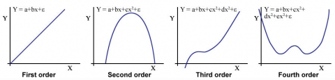
A set of functions that can be useful for describing quantitative responses are the various orders of polynomial functions. Polynomial functions have a general form:
[latex]Y=a + bx + cx^2 + dx^3 + ... + nx^{n-1} + \epsilon[/latex].
[latex]\textrm{Equation 9}[/latex] Polynomial function model.
A horizontal line is a polynomial function of order 0. Linear relationships are polynomial functions of the first order. The highest exponent of X in the function determines the order of the polynomial (0 for a horizontal line, 1 for simple linear regression equation). Each order has a distinctive shape. First-order polynomials produce a straight line, second-order polynomials produce a parabola, third-order polynomials produce a parabola with one inflection point and fourth-order polynomials produce a parabola with 2 inflection points. Graphs of the first 4 orders are shown Fig. 2 below.
Ex. 4, Non-Linear Regression and Model Comparison (4)
As with the other functions, an infinite number of curves may be created by carrying the coefficients. A polynomial function can usually be fit to most sets of data. The value of such relationships can be questioned at very high orders, though. Important in most functional relationships is the physical or biological relationship represented in the data. Higher-order relationships sometimes produce detailed equations which have a relatively limited physical or biological relevance.
ADDING ORDERS OF FUNCTIONS
Polynomial relationships are calculated to reduce the variability around the regression line, whatever the order. The usual technique is to begin with a linear equation. If the deviation from this line is significant, add a term to reduce the sum of squares (SS) about the line. Adding another order to the polynomial reduces the sum of squares. When the reduction of the sum of squares by adding another order becomes small, the limit of the equation has been reached. Enough terms can be added to fit any dataset. Generally, a third-order equation is the upper limit of terms in an equation to have any relevance. More terms often simply fit the error scatter of the data into the equation without adding additional relevance.
Ex. 4, Non-Linear Regression and Model Comparison (5)
Each additional order should be tested for significance using the hypothesis H0: highest order coefficient = 0. This can be tested using the equation:
[latex]\small F={\dfrac{\text{Regression SS for higher degree model - Regression SS for lower degree model}}{\text{ Residual MS for higher degree model}}}[/latex].
where:
[latex]\small \textrm{Numerator df}[/latex] = 1,
[latex]\small \textrm{Denominator df}[/latex] = residual df for the higher order model.
Test additional models using the same approach.
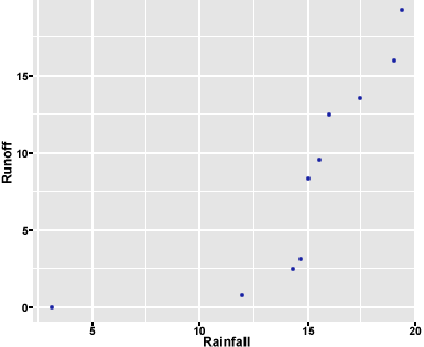
Now we’ll look at some very simple data and try to find the best model to fit the data. In the file QM-Mod13-ex4.csv, you’ll find a very small data set giving the rate of runoff for various amounts of rainfall. Read the file QM-Mod13-ex4.csv into R and take a look at it (there are only 10 entries, so don’t use the “head” command).
data<-read.csv(“ex4.csv”,header=T)
data
Ex. 4, Non-Linear Regression and Model Comparison (6)
R returns
Rainfall Runoff
1 3.00 0.00
2 12.00 1.00
3 14.00 2.50
4 14.50 3.25
5 15.00 8.50
6 15.50 9.50
7 16.00 12.50
8 17.50 13.50
9 19.00 16.00
10 19.25 19.00
Let’s plot the data quickly to see if we visualize any obvious trends.
library(ggplot2)
gplot(data=data,x=Rainfall,y=Runoff)
Ex. 4, Non-Linear Regression and Model Comparison (7)
R returns the plot in Fig. 3.
Let us run the regression models of the 1st and 2nd order (i.e. Runoff ~ Rainfall and Runoff ~ Rainfall^2) and compare them visually and statistically. We will plot the predictive function given by each regression model output on a scatterplot with these data and compare the models visually.
We use “I” in front of the “x” variable in the “lm” command to indicate to R that we want the higher-order of x included in the model (i.e., for a second-order model, we would indicate x2 by entering: I(x^2).
Ex. 4, Non-Linear Regression and Model Comparison (8)
Enter the models into the R console. Call the “Rainfall” variable x, and the “Runoff” variable y.
x<-data$Rainfall
y<-data$Runoff
m1<-1m(y~x,data-data) #1st order
m2<-1m(y~x+I(x^2),data=data) #2nd order
m3<-1m(y~x+I(x^2)+I(x^3),data=data) #3rd order
Here, we create the points on the line or parabola given by each model. Because the distance between these points is so small, they will appear as a line on our figure.
1d<-data.frame(x=seq(0,20,by=0.5))
result<-1d
result$m1<-predict(m1,newdata=1d)
result$m2<-predict(m2,newdata=1d)
result$m3<-predict(m3,newdata=1d)
Ex. 4, Non-Linear Regression and Model Comparison (9)
Here, we use the package “reshape2” to change the format of the data to facilitate graphing in the next step.
library(reshape2)
library(ggplot2)
result<-melt(result,id,vars=”x”,variable.name=”mode1″,value.name=”fitted”)
names(result)[1:3]<-c(“rainfall”,”order”,”runoff”)
levels(result$order)[1:3]<-c(“1st”,”2nd”,”3rd”)
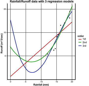
Finally, we are ready to plot the 1st, 2nd, and 3rd order regression models on top of the original data.
ggplot(result,aes(x=rainfall,y-runoff))+
theme bw()+ggtitle(“Rainfall/Runoff data with 3 regression models”)+
geom point(data=data,aes(x=x,y=y))+
xlab(“Rainfall (mm)”)+
ylab(“Runoff(m^3/sec)”)+
geom line(aes(colour=order),size=1)
Ex. 4, Non-Linear Regression and Model Comparison (10)
R returns the plots for the different-order polynomials in a single graph (Fig. 4).
1ST ORDER MODEL
Let’s take a look at the output for the 1st-order regression model and ANOVA.
summary(m1)
anova(m1)
Ex. 4, Non-Linear Regression and Model Comparison (11)
R outputs,
Call:
lm(formula = y ~ x, data = data)
Residuals:
Min 1Q Median 3Q Max
-5.4079 -3.5828 0.6918 2.2866 5.0015
Coefficients:
Estimate Std. Error t value Pr(>|t|)
(Intercept) -8.3336 4.5632 -1.826 0.10524
x 1.1601 0.2997 3.871 0.00473
(Intercept)
x **
—
Signif. codes: 0 ‘***’ 0.001 ‘**’ 0.01 ‘*’ 0.05 ‘.’ 0.1 ‘ ‘ 1
Residual standard error: 4.174 on 8 degrees of freedom
Multiple R-squared: 0.6519,
Adjusted R-squared: 0.6084
F-statistic: 14.98 on 1 and 8 df, p-value: 0.004735
Ex. 4, Non-Linear Regression and Model Comparison (12)
Analysis of Variance Table
Response: y
Df Sum Sq Mean Sq F value Pr(>F)
x 1 261.11 261.105 14.984 0.004735
Residuals 8 139.40 17.425
—
Signif. codes: 0 ‘***’ 0.001 ‘**’ 0.01 ‘*’ 0.05 ‘.’ 0.1 ‘ ‘ 1
The equation given by the linear model is yRunoff = -8.3336 + 1.1601xRainfall. The intercept is not statistically significant; the x variable is. The r2 value is 0.6519, and the linear regression is significant, but there is scatter about the regression line. The ANOVA shows a regression SS of 261.11 and a residual SS of 139.4 for the 1st-order model (Fig. 4).
Ex. 4, Non-Linear Regression and Model Comparison (13)
2ND ORDER MODEL
summary(m2)
anova(m2)
R outputs,
Call:
lm(formula = y ~ x + I(x^2), data = data)
Residuals:
Min 1Q Median 3Q Max
-2.512 -1.558 0.205 1.189 3.292
Coefficients:
Estimate Std. Error t value Pr(>|t|)
(Intercept) 4.20020 3.44216 1.220 0.26189
x -1.87695 0.63627 -2.950 0.02141 *
I(x^2) 0.13687 0.02785 4.915 0.00172 **
—
Signif. codes: 0 ‘***’ 0.001 ‘**’ 0.01 ‘*’ 0.05 ‘.’ 0.1 ‘ ‘ 1
Residual standard error: 2.115 on 7 degrees of freedom
Multiple R-squared: 0.9218,
Adjusted R-squared: 0.8995
F-statistic: 41.26 on 2 and 7 df, p-value: 0.0001337
Ex. 4, Non-Linear Regression and Model Comparison (14)
Analysis of Variance Table
Response: y
Df Sum Sq Mean Sq F value Pr(>F)
x 1 261.105 261.105 58.363 0.0001222 ***
I(x^2) 1 108.085 108.085 24.160 0.0017229 **
Residuals 8 31.316 4.474
—
Signif. codes: 0 ‘***’ 0.001 ‘**’ 0.01 ‘*’ 0.05 ‘.’ 0.1 ‘ ‘ 1
Here you can see that the R2 value increased, indicating that more of the variance in the data is explained by the regression equation. Testing the reduction using the F-test produces a very significant decrease in unexplained variability as the residual SS drops from 139.4 to 31.316. The regression line (green parabola) follows the data closely (Fig. 4).
Ex. 4, Non-Linear Regression and Model Comparison (15)
3RD ORDER MODEL
Let us take a look at the output for the 1st order regression model and ANOVA.
summary(m3)
anova(m3)
Call:
lm(formula = y ~ x + I(x^2) + I(x^3), data = data)
Residuals:
Min 1Q Median 3Q Max
-2.7284 -1.2079 0.3878 1.1311 2.4531
Coefficients:
Estimate Std. Error t value Pr(>|t|)
(Intercept) 15.51888 10.04750 1.545 0.173
x -6.94363 4.28634 -1.620 0.156
I(x^2) 0.63545 0.41826 1.519 0.180
I(x^3) -0.01393 0.01166 -1.195 0.277
Residual standard error: 2.053 on 6 degrees of freedom
Multiple R-squared: 0.9368
Adjusted R-squared: 0.9052
F-statistic: 29.66 on 3 and 6 df, p-value: 0.0005382
Ex. 4, Non-Linear Regression and Model Comparison (16)
Analysis of Variance Table
Response: y
Df Sum Sq Mean Sq F value Pr(>F)
x 1 261.105 261.105 61.9225 0.0002229 ***
I(x^2) 1 108.085 108.085 25.6330 0.0023041 **
I(x^3) 1 6.017 6.017 1.4269 0.2773480
Residuals 8 25.300 4.217
—
Signif. codes: 0 ‘***’ 0.001 ‘**’ 0.01 ‘*’ 0.05 ‘.’ 0.1 ‘ ‘ 1
Here, you see that not much more information about the response has been gained. The R2 (and R2Adj) increases little, and very little additional variability is explained in the third-order regression (Fig. 4). In the ANOVA table, the F-value for the third-order regression is not significant at even the 0.10 level. The second-order polynomial, therefore, is the best polynomial equation for describing the response. Physically, we are trying to fit a relationship between rainfall to runoff. The negative runoff or infiltration after rain begins makes sense. The x2 relationship may be explainable since we are considering a volume of runoff from a depth of rainfall. The equation does fit the data well. Again, this fits only the data gathered. Use of this relationship beyond the scope of this dataset would be improper.
Problems in Multiple Regression
Examining Problems
Recall the assumptions for regression discussed at the beginning of the lesson and in Chapter 10 on Mean Comparisons. If the assumptions necessary for multiple regression are not met, a number of problems can arise. These problems can usually be seen when examining the residuals, the difference between the actual Y’s and the predicted Y’s.
First, if the Y’s are not independent, serial correlation or auto-correlation problems can result. These can be seen if the residuals are plotted versus the X values, showing a consistently positive or negative trend over portions of the data. When collecting data over a period of time, this can be a problem since temporal data has some relationship to the value at the previous time. For instance, a temperature measurement 5 minutes after a previous one is going to be strongly correlated with the previous measurement because temperatures do not change that rapidly. These problems can be overcome by analyzing the data using different techniques. One of these is to take the difference of the value at the current time step from the value at the last time step as the Y value instead of the measured value.
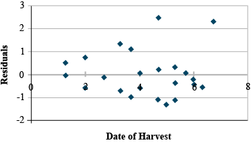
Second, violating the equal variances assumption leads to heteroscedasticity. Here the variance changes for changing values of X. A plot of residuals where the spread gradually increases toward lower or higher X’s can also occur. The residual plot from the replicated data regression in Chapter 7 on Linear Correlation, Regression and Prediction shows a hint of this. Notice how the residuals start to spread slightly as date of harvest, X, increases (Fig. 5).
Multicollinearity

The third problem is multicollinearity, as we discussed in the first part of the unit. Here two or more independent variables (x) are strongly correlated (for example, the GDD and hours of sunlight variables). The individual effects are hard to separate and lead to greater variability in the regression. Large R2 values with insignificant regression coefficients are seen with this problem. Eliminating the least significant variable after testing will often solve this problem without changing the R2 very much. The example just discussed showed such a property, where the X1 and X2 values were strongly correlated (r=.905). The insignificant coefficient can be eliminated, usually solving the problem (Fig. 6).
Polynomial Relationships
The application of the various orders of polynomial functions in describing quantitative responses has been covered in the earlier section – Polynomial Functions above. The equations, which are linear in the parameters (a, b, c, in Equation 9), are used to fit experimental data similar to the methods described earlier in this unit. Also covered earlier is enough terms can be added to fit any data set, with, in general, a third-order equation being the upper limit of terms in an equation to have any relevance. More terms often simply fit the error scatter of the data into the equation without adding additional relevance.
Each additional order should be tested for significance using the hypothesis H0: highest order coefficient = 0 using the F-test equation in section (Ex. 4. Non-Linear Regression and Model Comparison (5)) above.
Polynomial Regression
Polynomial Example
Let’s use the example from Chapter 7 on Linear Correlation, Regression and Prediction. The data set was approximated using a linear model (Fig. 7).
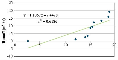
The R2 value is 0.62, with a regression SS of 242.1 and a residual SS of 149.2. The linear regression is significant, but there is a scatter about the regression line. Fitting the same data with a second-order polynomial produces:
| n/a | df | SS | MS |
|---|---|---|---|
| Regression | 2 | 362.2 | 181.10 |
| Residual | 7 | 29.1 | 4.15 |
| Total | 9 | 391.3 | n/a |
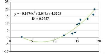
[latex]\small y = 4.32 - 2.05x + 0.15x^2[/latex].
[latex]r^2 = \small 0.93[/latex].
[latex]\small F=\frac{362.2-242.1}{4.15} = \small 28.9[/latex].
[latex]\small \textrm{Critical F} = \textrm{12.25; p-value = 0.01}[/latex].
[latex]\small \textrm{with df 1, 7}; p-value {\lt \lt \lt 0.01}[/latex].
Variance in the Data
Here you can see that the R2 value increased, indicating that more of the variance in the data is explained by the regression equation. Testing the reduction using the F-test produces a very significant decrease in unexplained variability as the residual SS drops from 149.2 to 29.1. The regression line follows the data closely (Fig. 8).
Going a step further to assure that most of the variance is explained by the regression equation, we fit a third order polynomial (Table 5).
| n/a | df | SS | MS |
|---|---|---|---|
| Regression | 3 | 365.6 | 121.90 |
| Residual | 6 | 25.7 | 4.28 |
| Total | 9 | 391.3 | n/a |
[latex]\small y = 12.14 - 5.94x^2 + 0.01x^3[/latex].
[latex]r^2 = \small 0.93[/latex].
[latex]\small F=\frac{365.6-262.2}{4.28} = \small 0.79[/latex].
[latex]\small \textrm{Critical F} = \textrm{3.29; p-value = 0.01}[/latex].
[latex]\small \textrm{with df 1, 7}; \textrm{not significant, even at p-value = 0.01}[/latex].
Calculating Polynomial Equations
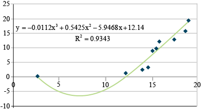
Here, you see that not much more information about the response has been gained. The R2 increases little, and very little additional variability is explained in the third-order regression (Fig. 9). The F-value for third-order regression is not significant at even the 0.10 level. The second-order polynomial, therefore, is the best polynomial equation for describing the response. Physically, we are trying to fit a relationship between rainfall to run-off. The negative run-off or infiltration after rain begins makes sense. The X2 relationship may be explainable since we are considering a volume of run-off from a depth of rainfall. The equation does fit the data well. Again, this fits only the data gathered. Use of this relationship beyond the scope of this data set would be improper.
R CODE FUNCTIONS
- anova
- summary
- lm
- install.packages
- library
- cor
- pcor
You are a maize breeder in charge of developing an inbred line for use as the ‘female’ parent in a hybrid cross. Yield of the inbred female parent is a major factor affecting hybrid seed production; a high level of seed production from the hybrid cross leads to more hybrid seed that can be sold. Only 3 lines remain in your breeding program, and your boss wants you to determine 1. Which is the best model to use to analyze the data, and 2. Which of the three lines should be selected for advancement in the breeding program? The three-variable data set relating the yield (per plot) of the 3 inbred lines (evaluated in 3 reps) to the amount of N and level of drought applied to each plot can be found in the file QM-mod13_ex5.csv.
Helpful questions to ask in writing the R code:
-
- Should “line” be classified as a numeric or factor variable?
- Should “rep” be classified as a numeric or factor variable?
- Should “rep” be included in the model?
- Should the interaction between N and drought be included?
- What higher orders of N and drought, if any, should be included in the model?
- Ex. 5: Non-Linear Multiple Regression Analysis (2)
Ex. 5: Non-Linear Multiple Regression Analysis (3)
The correct model is: yield ~ N + drought + line + rep + N*drought + N2 + drought2 “rep” and “line” should be factors, as the numeric values (1 to 3) are identifiers only and don’t indicate a treatment amount.
The model including drought and N as a 2nd-order variable is the best. The model that has drought as a 2nd order polynomial and N as a 3rd order polynomial technically has a better R2Adj, however since the difference between the R2Adj values of the 2 models is incredibly small AND since the coefficient N2 is not significant in the model with the higher-order polynomial, we choose the simpler of the 2.
data$line<-as.factor(data$line)
data$rep<-as.factor(data$rep)
summary(1m(data,yield~N+drought+line+rep+N*drought+I(N^2)+I(drought^2)))
Ex. 5: Non-Linear Multiple Regression Analysis (4)
R outputs,
Call:
lm(formula = yield ~ N + drought + line + rep + N * drought + I(N^2) + I(drought^2), data = data)
Residuals:
Min 1Q Median 3Q Max
-2872.09 -550.53 11.45 517.71 2123.26
Coefficients:
Estimate Std. Error t value Pr(<|t|)
(Intercept) 7.997e+03 9.944e+01 80.422 < 2e-16 ***
N 6.936e+01 1.504e+00 46.120 < 2e-16 ***
drought 7.172e+02 2.118e+01 33.864 < 2e-16 ***
line2 6.026e+02 7.264e+01 8.296 5.31e-16 ***
line3 8.256e+02 7.264e+01 11.366 < 2e-16 ***
rep2 -2.080e+02 7.264e+01 -2.864 0.00431 **
rep3 -8.158e+02 7.264e+01 -11.231 < 2e-16 ***
I(N^2) -2.730e-01 6.454e-03 -42.296 < 2e-16 ***
I(drought^2) -1.920e+02 5.069e+00 -37.869 < 2e-16 ***
N:drought 4.716e-01 1.587e-01 2.971 0.00306 **
—
Signif. codes: 0 ‘***’ 0.001 ‘**’ 0.01 ‘*’ 0.05 ‘.’ 0.1 ‘ ‘ 1
Residual standard error: 800.7 on 719 degrees of freedom
Multiple R-squared: 0.9211, Adjusted R-squared: 0.9201
F-statistic: 933.1 on 9 and 719 df, p-value: < 2.2e-16
Ex. 5: Non-Linear Multiple Regression Analysis (5)
anova(m2)
Analysis of Variance Table
Response: yield
Df Sum Sq Mean Sq F value Pr(>F)
N 1 254135518 254135518 396.4202 < 2.2e-16 ***
drought 1 2881646910 2881646910 4495.0156 < 2.2e-16 ***
line 2 88656727 88656727 69.1468 < 2.2e-16 ***
rep 2 87339382 87339382 68.1194 < 2.2e-16 ***
I(N^2) 1 1146830086 1146830086 1788.9142 < 2.2e-16 ***
I(drought^2) 1 919337101 919337101 1434.0531 < 2.2e-16 ***
N:drought 1 5659813 5659813 8.8286 0.003064 **
Residuals 719 460933695 641076
—
Signif. codes: 0 ‘***’ 0.001 ‘**’ 0.01 ‘*’ 0.05 ‘.’ 0.1 ‘ ‘ 1
Line 3 has the best predicted yield and should be advanced.
Summary
Multiple Regression
- Effects of several continuous independent variables (Xs) on continuous dependent variable Y
- With just X1 and X2, get the plane of best fit.
Multiple Correlation
- Start with all pairwise simple correlations of Y and Xs.
- Partial correlation of Y and X1 holds all other Xs at their average value.
- Total multiple correlation of Y on Xs squared (R2) is the coefficient of determination
Calculating Multiple Regression
- In R, use the REG procedure
- Get prediction equation Y = a + b1X1+…+bkXk from Parameter Estimates
- Get Analysis of Variance for Regression
Testing Multiple Regression
- R2 gives the proportion of variation accounted for by Regression
- Overall F-test of all coefficients equal to zero
- Each regression coefficient tested in Parameter Estimates or Effect Tests
Problems in Multiple Regression
-
- Ys not independently distributed
- Unequal variances
- Either of these is seen in residual plots
- Multicollinearity from high pairwise correlations of Xs
Polynomial Regression
- Add successive powers of X: X, X2, X3, …
- Test for significance with F-test.
How to cite this chapter: Mowers, R., D. Todey, K. Moore, L. Merrick, A. A. Mahama, & W. Suza. 2023. Multiple Regression. In W. P. Suza, & K. R. Lamkey (Eds.), Quantitative Methods. Iowa State University Digital Press.
The simple correlation explains how well correlated a single Xi and the resulting Y are in a multiple correlation. This simple correlation ignores any understanding of correlation between the Xi involved and another Xi. It is calculated similar to a regular correlation.
Partial correlation displays the numerical relationship between a single Xi and Y in multiple correlation. In contrast to the simple correlation, the partial correlation accounts for interaction between the Xi's and illustrates the true relationship between the Xi and Y.
The multiple correlation coefficient displays the numerical linear relationship between a several Xi's and Y in multiple correlation. This enumerates the total relationship between the combined effects of the Xi's and the resulting Y.
