Some types of data are measured in discrete units. For example, we might count the number of insects on a plant or the number of plants in a segregating population with a transgene.

In this chapter, we will concentrate on binomial data, which are characterized by having only two possible states, for example, germinated or not germinated in a seed germination experiment. Other examples are cornstalks which are either stalk lodged or not, plants diseased or not, and survey data in which farmers either agree or disagree with an issue.

Definition of Binomial

A fixed number of independent trials, each with two outcomes and constant proportion of success, follow the binomial distribution. Not all data we wish to analyze are from a normal distribution. As we saw in unit one, some variables have discrete values. For this unit and the next, we analyze data which are discrete or categorical.

The first type we analyze are data which arise from a Bernoulli trial, i.e., two possible outcomes. They are characterized by four requirements: two outcomes for each trial, a fixed number of trials, independent trials, and a constant probability of success on each trial. These types of trials give rise to the binomial distribution. The true probability of success, designated p is one parameter of the binomial distribution. The probability of failure is q = 1 – p. For example, in a seed germination experiment, we only have two outcomes for each seed: either it germinates or fails to germinate.

The use of p to represent the proportion of successes does not adhere to the usual convention of using Greek letters for parameters. Some texts use the symbol π for the parameter, but we will use p because it is widely used in population and quantitative genetics. Do not confuse this p with the use of P as a probability statement. Your discernment will need to be based on context rather than memorization.

Another Binomial Situation

For the binomial distribution, there is a fixed number (n) of independent trials for which we count the number of successes. n represents the second parameter of the binomial distribution. In germination tests, we often use n = 100 seeds. These trials are assumed to be independent; where if one seed germinates, it does not affect whether another seed will germinate. We also assume there is a constant true germination proportion (p) for any seed in the seed lot.

Another example of a binomial situation is root lodging counts in corn yield trial plots. There are 60 plants per plot planted with a precision planter, and each plant can be considered an independent trial with two possible outcomes, root lodged or not. We assume that there is a constant genetic proportion of a root lodged plant (“success”) for any of the individual plants (trials). The inherent genetic susceptibility to root lodging is considered a characteristic of a corn hybrid, and we want to estimate the proportion, p, which will root lodge. We count the number of lodged plants per plot and use those data for determining differences among corn hybrids.

To determine if you are in a binomial situation, there are four requirements:

1. There should be two outcomes for each trial (S or F, 0 or 1, etc.).
2. There should be a fixed number of trials.
3. Each trial should be independent of the others.
4. There is a true proportion of success, p, which is the same for each observation or trial.

Assumption of Independence

You might wonder how often the assumption of independence is violated in the same way as our example of drawing cards from a deck without replacement. For example, if a seed salesman wishes to survey 40 of his 650 customers with a yes-no question, does he violate the assumptions necessary for using the binomial distribution?

In general, if our sample is 10%, or less, than the size of the target population, and all other assumptions are met, we can use the binomial distribution results. Otherwise, we need to adjust the standard errors using a finite population correction factor, an adjustment found in some statistics textbooks, but not covered here.

Do not restrict your sample size just to be able to use the binomial distribution if, for example, it is necessary to sample, say 100 of the 650 salesmen to get precise results. Get the sample size adequate for the precision you need, and then, if needed, get help from a statistician to analyze the data.

Discussion

Do you think that all the assumptions of a binomial situation are valid for the number of lodged plants per plot? Why or why not?

The Binomial Probability Function

Calculate Probabilities

A formula allows us to calculate probabilities for binomial data. Generally, we are interested in two types of questions for a binomial experiment. One is the number of successes in the n independent trials. We might want to know how often the count of the number of “successes” is greater than a given value. For example, if the count is the number of dead insects from a set of 25 corn rootworms fed on transgenic root tissue, we may want to know how often we observe fewer than 16 dead if the true proportion which die is p = 0.9.

A second important question is how to estimate p, the true proportion of successes. This parameter p is the true average number of successes divided by n. For example, if the true average for the entire population is that 21 of the 25 insects die when fed the tissue (in other words, for all possible sets of 25 test insects fed this tissue, an average of 21 will die), the true proportion of success is p = 0.84. We will see in the next section how to estimate p from a sample.

The formula for answering the first question is as follows. If s is the number of successes in n independent trials for the binomial situation, the probability that s is a given value k is:

[latex]P_{(s=k)} ={\dfrac{n!}{k!(n-k)!}}p^kq^{(n-k)}[/latex]

[latex]\text{Equation 1}[/latex] The Binomial Distribution Formula,

where:
[latex]n[/latex] = number of trials,
[latex]q[/latex] = 1-p,
[latex]k[/latex] = any integer between zero and n, representing the number of successes in the trial.

Recall that a factorial (denoted by !) is calculated as: n!=n*(n-1)*(n-2)*…2*1. How do we use this formula? Suppose we sample 10 plants, each with true probability 0.25 of containing a Bt gene. Leaf samples from each of the plants are evaluated with an error-free diagnostic test for the gene. Assume these plants are a random sample of a large number of plants. What is the probability that we get 2 of 10 samples that are positive for the gene?

First, think, “Is this a binomial situation?” There are two outcomes: either the gene is present in a plant or not. There are 10 independent trials because if any plant has the gene, that does not affect whether another plant does. We can also assume that there is constant genetic proportion of plants with the gene, p = 0.25. This does fit the binomial situation.

To calculate the probability that two plants will have the gene, substitute into the formula to find:

[latex]P_{(s=2)} ={\dfrac{10!}{2!(10-2)!}}0.25^2*0.75^{(10-2)}[/latex]

[latex]P_{(s=2)} ={\dfrac{10!}{2!(8)!}}0.25^20.75^{(8)}[/latex]

[latex]P_{(s=2)} ={\dfrac{10*9*8*7*6*5*4*3*2*1}{2*1(8*7*6*5*4*3*2*1)}}0.25^20.75^{(8)}[/latex] = (45)(0.625)(0.100113)=0.2816.

[latex]\text{Equation 2}[/latex] Calculating the probability using the Binomial Distribution Formula.

This is the probability of getting 2 positives.

Try This! Probability Exercises

Ex. 1: Binomial Probabilities (1)

In this exercise, we use Excel to get probabilities for the number of successes as shown in Equation 1. We will also illustrate the difference between the Binomial Distribution and Binomial Probability functions.

We will create a table of probabilities for an experiment with n=10 independent trials and p=0.25. We will get probabilities for each number of successes possible for this experiment, 0, 1, . . . , 10. We will also get the binomial distribution cumulative probabilities for numbers of successes less than or equal to each of these values.

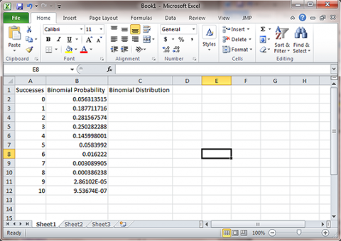
1. Open a new Excel workbook and label three columns: Successes, Binomial Probability and Binomial Distribution. Under Successes, fill in successive integers 0-10 (Fig. 1).
2. Enter the formula “=Binom.dist(A2, 10, 0.25, False)” in the cell next to zero under Binomial Probability. A2 refers to the cell with the number of successes, 10 is the number of trials, p=0.25, and False indicates that the Probability Mass Function should be used. This means that Excel returns the probability of each success in Column A. If we instead set the last parameter of “=Binom.dist” to True, Excel calculates the combined probability of all successes of s or lower. For example, the probability of 2 successes would also include the probability of 1 or 0 successes. Now, copy that formula into the next ten cells in the Binomial Probability column.

Ex. 1: Binomial Probabilities (2)

3. This gives the probability for each possible number of successes (k). For example, k=2 successes has 0.2816 probability of occurring.
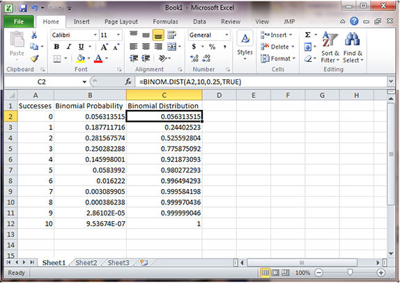
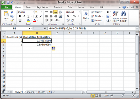
4. To get the cumulative probabilities, for the third column, enter the formula “=Binom.dist(A2, 10, 0.25, TRUE)”.

This gives the table to the right. Notice that the probability for 2 or fewer successes is 0.5256, as we computed in Study Question 4.

Ex. 2: Table of Probabilities

In this exercise we use Excel to reconstruct a column of the table of probabilities. For this we use p = 0.4, n=6, and the number of successes as shown in the middle column of the table (Fig. 2).

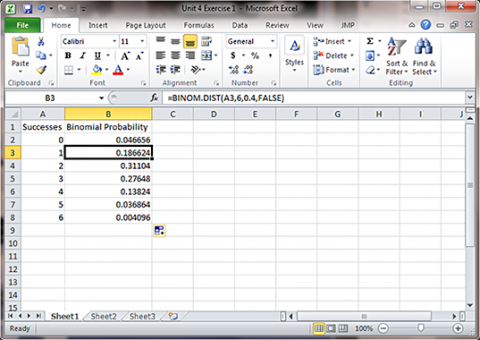
1. Open a new Excel workbook. Follow the same steps for Binomial Probability, but the number of successes is 6 and p=0.4. The formula to use is “=Binom.dist(A2, 6, 0.4, FALSE)”.
2. This gives the probability for each possible number of successes (k). For example, k=3 successes has 0.2765 probability of occurring.

Ex. 3: Cumulative Binomial Probability

In this exercise, we use Excel to solve a probability question. The question asks for the probability of 7 or fewer successes in 15 trials with p=0.4. Because we need a cumulative probability, we use the Binomial Distribution function with p = 0.4, n=15, and k=7 (Fig. 3).

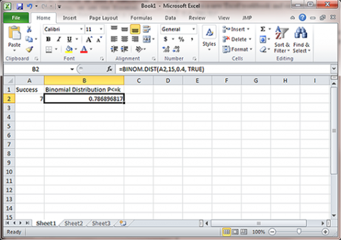
Open a new Excel workbook and enter the number of successes as 7. This exercise calculates the cumulative probability, so the formulas “=Binom.dist(A2, 15, 0.4, TRUE)”

This gives the probability for each possible number of successes (k). For our example, k=7 or fewer successes has 0.7869 probability of occurring. Notice that the Excel Binomial Distribution function gives the cumulative probability based on a binomial distribution rather than a normal approximation (0.7852).

Ex. 4: Probability Computations

In this exercise, we use Excel to exactly solve a more complicated probability question. This question asks for the probability of between 4 and 6 successes in 10 trials with p=0.25. The probability of between 4 and 6 successes is the probability of 6 or fewer successes minus the probability of 3 or fewer successes. Because we need to use cumulative probabilities, we use the Binomial Distribution function with p = 0.25, n=10, and k=3 or 6 (Fig. 4).

This function gives, in the second column, the cumulative probability for each possible number of successes (k). For our problem, k=3 or fewer successes has 0.7759 probability of occurring, and k=6 or fewer successes has probability 0.9965 of occurring. We subtract these, P(k<=6) – P(k<=3) or 0.9965 – 0.7759 = 0.2206, the probability of between 4 and 6 successes occurring.

The Mean and Variance

Mean and Variance

The number of successes [latex]s[/latex] for a binomial distribution has mean [latex]np[/latex] and variance [latex]npq[/latex]:

For number of successes, s:
Mean = [latex]np[/latex]
Variance = [latex]npq[/latex]

The sample proportion in a binomial distribution, [latex]\hat{p}=\frac{s}{n}[/latex], has mean and variance:

For the sample proportion,  :
Mean = [latex]p[/latex]
Variance = [latex]\frac{pq}{n}[/latex].

Suppose we have binary data for root lodging with true proportion lodged, p = 0.08 and n = 60 plants per plot. The true average number of root lodged plants in a plot is 4.8 and the variance is 4.4. In other words, we expect to count about five lodged plants per plot, and have standard deviation of about two plants per plot (std = sqrt(4.4) = 2.09).

Standard Deviations

One problem not yet discussed with the example of root lodging is that although the variable itself may be considered to follow a binomial distribution with constant genetic proportion of lodged plants, there are other sources of variation. Field, disease, weather-related, and other variation will add to the variation of root lodging in a real situation. Our standard deviations are likely to be much greater when you consider mistakes in counting, the variation of soils in the yield trial field area, and the variations in thunderstorm wind speed throughout the yield trial location. The binomial variance gives us the inherent variation in lodging counts, but there are other sources of error that will inflate the estimated variance of a population.

The variance for the sample proportion can be computed if we know p, and the maximum variance is when p = 0.50. As an example, suppose our objective is to estimate the germination percentage from a sample of 100 seeds. If the true germination proportion for the seed lot is 0.95, what is the variance for , our sample estimator of ? The variance of p is 0.95*0.05/100 = 0.000475. The standard deviation is 0.022, or 2.2% germination. If the true proportion is 0.80 and we have 100 seeds, the variance is 0.80*0.20/100 = 0.0016, and the standard deviation is 0.04, or 4% germination. The maximum variance of p will occur when = q = 0.50, and is 0.50*0.50/100 = 0.0025. The standard deviation is 0.05, or 5% germination.

Estimating Trial Numbers

The previous study question illustrates a method for finding the number of trials, n, needed to achieve a certain level of precision for estimating p in a binomial situation. We know the maximum variance will occur when p = 0.5, and we can solve to get:

[latex]n=\frac{pq}{v}[/latex]=[latex]n=\frac{0.5*0.5}{v}[/latex]=[latex]n=\frac{0.25}{v}[/latex]

[latex]\text{Equation 3}[/latex] Formula for estimating trial numbers,

where:
[latex]n[/latex] = minimum number of trials,
[latex]p[/latex] = proportion of successes,
[latex]q[/latex] = 1-p,
[latex]v[/latex] = variance.

This is a conservative estimate because we are using the maximum variance of our estimator. If we knew more about the true proportion p, for example, 0.30, we would use the formula n = 0.3*0.7/ v.

The Normal Approximation

Approximate the Binomial

It is an interesting phenomenon that the histogram for the number of successes in a binomial distribution looks like the normal distribution, especially if n is large and p is not too close to either zero or one. In fact, the normal distribution can be used as an approximation to the binomial.

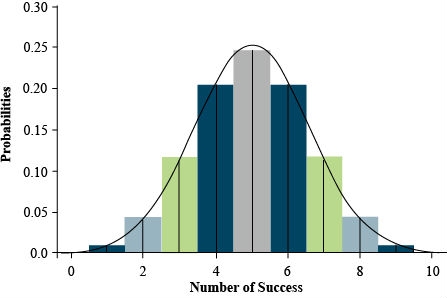
Figure 5 shows the correspondence of the histogram of a binomial distribution to the frequency curve of the normal distribution. This is for a binomial distribution with n = 10 trials and p = 0.5. For this case, the normal curve passes very closely to the center of each bar of the binomial histogram. Even if p is not 0.5, if n is large, the normal curve can approximate the binomial.

Normal Approximation

We see from Fig. 5 that probabilities under the normal curve will better approximate the histogram for the binomial distribution if we measure the area for s values less than k + 0.5. For example, to sum the area of 0, 1, and 2 successes, we would add the probabilities (areas of bars) for binomial, and this area is better approximated by the area under the normal curve less than s = 2.5. If we just use the probability for the normal less than k, we would miss half the bar representing the probability in the binomial histogram. Therefore, P_Binomial(s ≤ k) is better approximated by the normal distribution using P_Normal(s < k + 0.5). This correction factor is used when the normal approximation can be used, but sample sizes are small.

The general rule to know when to use the normal approximation is to use it for the number of successes in a binomial distribution when the mean (np) is not too close to zero or one. Specifically, we use the normal approximation when (np ≥ 5) and (nq ≥ 5).

You might wonder why we should use the normal approximation at all when we can use computer programs to compute exact probabilities for the binomial distribution. With the normal approximation, we can sometimes do confidence intervals much more easily, for example using the mean plus or minus two standard deviations for an approximate 95% confidence interval. We will also see that we can employ a normal approximation for testing hypotheses about proportions or comparing proportions from independent samples.

Conclusions from the Example

In this example we have a case that requires us to use the exact binomial distribution. The value of p is so small that np < 5, and it is necessary to use the exact binomial distribution.

What can we conclude from the situation in study question 8 if we ran our test and found the 600-seed sample to be negative (no transgenic event present)?

Using Equation 1, we calculate that the exact probability for no positives in a sample of 600 is:

P₀ = (1)(0.001)⁰(0.999)⁶⁰⁰ = (0.999)⁶⁰⁰ = 0.549

The value is not at all unusual if our null hypothesis is H₀: p = 0.001. Our sample is in concert with this null hypothesis. However, if our null hypothesis is that p is 0.005, the probability of observing no transgenic event in a sample of 600 is (0.995)⁶⁰⁰ = 0.049. Thus, it is unlikely that the amount of contamination is as high as 0.005 (a half percent).

We have used our rule of thumb (np and nq ≥ 5 for normal approximation) to dictate that we need the exact binomial distribution. However, we also would not use the normal approximation in problems where there are severe consequences if we get the probabilities wrong.

Computing a Probability

If we germinate 400 seeds and the true percent germination is 95%, we can use the book’s Appendix 1 table to compute the probability of observing a sample with less than 93% germination. We only use this example as an illustration because Excel can compute the probability more accurately with the binomial distribution.

Compute the mean and standard deviation as

[latex]{np}=400(0.95)=380, {}\text{}and \sqrt{npq}=\sqrt{4000*950*0.05}=436[/latex],

[latex]\text{Equation 4}[/latex] Formula for computing mean and standard deviation.

Observing 93% or fewer is observing 0.93*400 = 372 or less. Then, the probability of 93% or less in our sample has [latex]Z=\frac{372+0.5-380}{4.36}=-1.72[/latex], and using the

normal approximation and Appendix 1, [latex]P(Z\lt -1.72)=P(Z\gt 1.72)=1.00-0.9573=0.043[/latex].

Sample Exercises

This example is somewhat complicated, so we illustrate how to do the same example with Excel.

Another example of how to use the normal approximation to compute probabilities is as follows. Suppose we run a germination test using 200 seeds, and assume the true p is 0.91. What is the probability that between 174 and 190 of the seeds germinate?

We can use the normal approximation because np = 182 and nq = 18. Our general method for computing the probabilities is to first draw a curve with the mean and standard deviation of the normal distribution. The mean is np = 182, and the standard deviation is √(npq) = 4.047. From the normal approximation, about 68% of the values should be between 178 and 186, and about 95% are between 174 and 190. We see in the next ‘Try This’ how to get the probability, but we can just estimate it. Notice that 174 is about 2 std below the mean, 190 is 2 std above the mean, and so the probability is about 0.95.

Try This: Use Excel to Compute the Binomial Probability 

Ex. 5: Compute the Binomial Probability

In this exercise we use Excel to exactly solve the probability of 93% or fewer seeds germinating in 400 trials with p=0.95. Because we need a cumulative probability, we use the Binomial Distribution function with p=0.95, n=400, and k=372. The value for k is from 93% of 400, or 0.93*400 = 372.

• Open Excel and enter the formula for a cumulative probability since the statistic of interest is 93% or fewer seeds. This formula is “=binom.dist(372, 400, 0.95, TRUE)”, (Fig. 6).

This gives the cumulative probability for each possible number of successes (k) from 0 to 372. For our example, k=372 or fewer successes has 0.048 probability of occurring .

Ex. 6: Compute the Binomial Probability

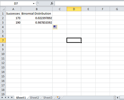
In this exercise, we use Excel to exactly solve a more complicated probability question. This question asks for the probability of between 174 and 190 successes in 200 trials with p=0.91. The probability of between 174 and 190 successes is the probability of 190 or fewer successes minus the probability of 173 or fewer successes. Because we need to use cumulative probabilities, we use the Binomial Distribution function with p = 0.91, n=200, and k = 173 or 190. Note the use of 173 rather than 174 to accommodate the entire interval (Fig. 7).

• This exercise uses the same technique as Exercise 4. Change the function so that it reflects p, n, and k for this problem.

This function gives, in the second column, the cumulative probability for each possible number of successes (k). For our problem, k=173 or fewer successes has 0.0224 probability of occurring, and k=190 or fewer successes has 0.9879 probability of occurring. We subtract these, P(k ≤ 190) – P(k ≤ 173) or 0.9879 – 0.0224 = 0.9655, the probability of between 174 and 190 successes occurring.

Reason to Use Normal Approximation

The reason we can use the normal approximation when p = 0.5, but not when p = 0.3 is that when p = 0.3, the binomial distribution is skewed. Even though our sample size is fairly small (12), if p = 0.5, the binomial distribution is symmetric and is better approximated by the symmetric normal distribution than when p = 0.3.

Confidence Intervals

Sample Proportion

The normal approximation allows us to compute confidence intervals for p.

If we have a normal distribution, a 95% confidence interval will be centered on the calculated average plus and minus two standard deviations. Note: A confidence interval is not the same as a confidence limit. The confidence interval contains a specified proportion of the distribution (e.g. 95%). The confidence limits are the endpoints of the confidence interval.

The sample proportion has true mean p and true variance pq/n. A 95% confidence interval for p is:

[latex]\hat{p}=\pm 1.96\sqrt{\frac{\hat{p}\hat{q}}{n}}[/latex]

[latex]\text{Equation 5}[/latex] Calculating confidence interval,

where:
[latex]\hat{p}[/latex] = sample proportion,
[latex]\hat{q}[/latex] = (1-p),
[latex]1.96[/latex] = number of standard deviations for a 95% confidence interval.

Confidence Interval Exercise

A confidence interval based on the approximation is easier to compute than the exact method, which is given in the ‘Try This!’ below. However, in some cases we need to use the method based on the exact binomial distribution, for example in computing a confidence interval for a proportion of plants contaminated with a genetically modified organism. Also, note that “exact” refers to the use of the binomial distribution rather than its normal approximation. We do not know “exactly” the value of the parameter p, but just provide an interval and have 95% confidence in the procedure to calculate it.

Testing Hypotheses

Testing for a Proportion

We can test hypotheses for a proportion using the normal approximation.

We wish to test the null hypothesis H₀ : p = p₀. We can do this with the normal approximation to the binomial. We can also do this with a more exact method based on the binomial distribution itself.

The test statistic for a large sample test is:

[latex]\frac{\hat{p}-\hat{q}}{\sqrt{\dfrac{p_{0}q_{0}}{n}}}[/latex]

[latex]\text{Equation 6}[/latex] Formula for testing proportion.

Here p₀ is the hypothesized value of p, [latex]\hat{p}[/latex]  is the estimate from the sample, and q₀ is (1 – p₀).

Try This 1: Use Excel to Test a Hypothesis for p

Ex. 8: Test the Hypothesis for p

For this example, we test whether 112 successes (purple-stemmed plants) of 158 total could fit the hypothesis of p=0.75. In the sample, there are 112 purple and 46 green to make the 158 total. We want to know if they could fit the ratio 3:1, or 0.75 purple. We can use Equation 8.

The hypothesis tested is:

• H₀: p = 0.75 and q = 0.25
• H_α: p ≠ 0.75 and q ≠ 0.25
• This hypothesis can be tested using a confidence interval. If p=0.75 falls within the confidence interval, we fail to reject the null. If it does not fall within the CI, we reject the null hypothesis.

Steps:

• Open Excel and enter the formula “=binom.dist(112, 158, 0.75, TRUE)”.
• Equation 8 covered finding a 95% confidence interval with the upper and lower values being associated with a probability of at most 0.025. If the probability associated with 112 purple in a sample of 158 and p=0.75 is greater than 0.025, then p=0.75 is within the confidence interval and we fail to reject the null hypothesis.

The probability is > 0.13 and we fail to reject the null hypothesis (Fig. 8).

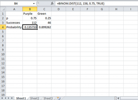
Notice that if you calculate the exact confidence interval for proportion purple (0.638, 0.779) it is the same as presented in the book. The confidence interval does include 0.75, and we fail to reject the null that p=0.75.

Try This 2: Use Excel to Test a Hypothesis for p

Ex. 9: Test the Hypothesis for p

For this example, we test whether 7 successes (cuttings which root) of 10 total could fit the hypothesis of p ≥ 0.9 (Fig. 9). We test the null that p ≥ 0.9 vs. the alternative that p is less than 0.9. This is a one-sided test, so the alpha level is 0.05, and is not divided by 2.

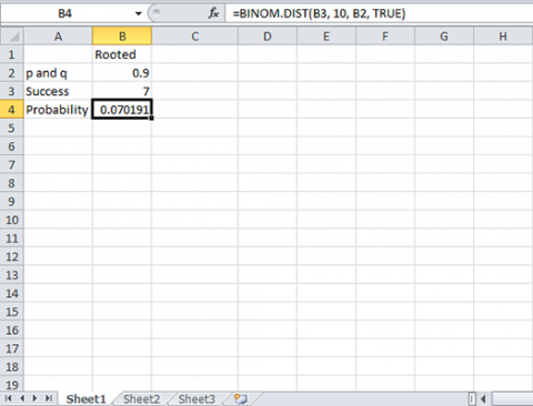
This is a one-sided hypothesis.

• H₀: p ≥ 0.9
• H_α: p < 0.9
• Open Excel and a new workbook.
• Enter the information from the image to the right.

Notice that the 90% confidence interval for proportion rooting is (0.493, 0.913). The probability value for the hypothesis test is P = 0.0702, which is not less than 0.05, so we fail to reject the null.

Comparing Proportions

In the same way that we can use the normal distribution to approximate the binomial for a single population, we can also approximate the binomial for two different populations. Thus, we can use the approximation for differences of proportions when we have two independent samples.

We can use this approximation to compute confidence intervals and test hypotheses for differences in proportions. The variance of a difference in two proportions is p₁q₁/n₁ + p₂q₂/n₂, which is just the sum of the variances from the two independent populations. Consequently, we compute a 95% confidence interval for p₁ – p₂ as:

[latex](\hat{p_1}-\hat{p_2})\pm1.96{\sqrt{\dfrac{\hat{p_1}\hat{q_1}}{n_1}+\dfrac{\hat{p_2}\hat{q_2}}{n_2}}}[/latex]

[latex]\text{Equation 7}[/latex] Formula for computing 95% confidence interval for p₁ – p₂.

Here, [latex](\hat{q})_1 = 1 - (\hat{p})_1[/latex]

and [latex](\hat{q})_2 = 1 - (\hat{p})_2[/latex]

This method of estimating a confidence interval for differences in proportions relies on large sample sizes and proportions not near 0 or 1. We do not give an example of hypothesis tests for differences in proportions because those are better done with contingency tables in the next unit.

Summary

Recognize the Binomial Situation

• Two outcomes.
• Fixed number of trials.
• Independent trials.
• Constant proportion of success

Binomial Probability

• Formula allows calculation.
• Excel computes probability or cumulative (Binomial Distribution).

Mean and Variance for Successes

• Mean = np, Variance = npq

Mean and Variance for Sample Proportion

• Mean = p, Variance = pq/n

Normal Approximation to Binomial

• Can use when np and nq ≥ 5.
• Helpful for approximate 95% Confidence Interval.

Estimate Confidence Intervals

• Exact Binomial method uses Excel.

Tests of Hypotheses

• For p = p₀ using Excel.
• For differences in proportions, see next chapter.